I've been trying to wrap my head around factor analysis as a theory for designing and understanding test and survey results. This has turned out to be another one of those fields where the going has been a bit rough. I think the key factors in making these older topics difficult are:

“Everybody knows this, so we don't need to write up the details.”
“Hey, I can do better than Bob if I just tweak this knob…”
“I'll just publish this seminal paper behind a paywall…”

The resulting discussion ends up being overly complicated, and it's hard for newcomers to decide if people using similar terminology are in fact talking about the same thing.

Some of the better open sources for background has been Tucker and MacCallum's “Exploratory Factor Analysis” manuscript and Max Welling's notes. I'll use Welling's terminology for this discussion.

The basic idea of factor analsys is to model $d$ measurable attributes as generated by $k < d$ common factors and $d$ unique factors. With $n = 4$ and $k = 2$ , you get something like:

Relationships between factors and measured attributes (adapted from Tucker and MacCallum's Figure 1.2)

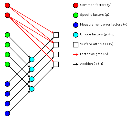
Corresponding to the equation (Welling's eq. 1):

(1)

x = A y + μ + ν

The independent random variables $y$ are distributed according to a Gaussian with zero mean and unit variance $𝒢_{y} [0, I]$ (zero mean because constant offsets are handled by $μ$ ; unit variance because scaling is handled by $A$ ). The independent random variables $ν$ are distributed according to $𝒢_{ν} [0, Σ]$ , with (Welling's eq. 2):

(2)

Σ \equiv diag [σ_{1}^{2}, \dots, σ_{d}^{2}]

The matrix $A$ (linking common factors with measured attributes $x) is refered to as the factor weights or factor loadings . Because the only source of constant offset is$ \mathbf{\mu} $, we can calculate it by averaging out the random noise (Welling' s eq . 6) : Unknown character div class = Unknown character numberedEq Unknown character Unknown character Unknown character span Unknown character (3) Unknown character / span Unknown character$ $μ = \frac{1}{N} \sum_{n = 1}^{N} x_{n}$ $Unknown character / div Unknown character where$ N $is the number of measurements (survey responders) and$ \mathbf{x}n $is the response vector for the$ n^\text{th} $responder . How do we find$ \mathbf{A} $and$ \mathbf{\Sigma} $? This is the tricky bit, and there are a number of possible approaches . Welling suggests using expectation maximization (EM), and there' s an excellent example of the procedure with a colorblind experimenter drawing colored balls in his [EM notes] [EM] (to test my understanding, I wrote Unknown character a href = Unknown character . / color - ball . py Unknown character Unknown character color - ball . py Unknown character / a Unknown character) . To simplify calculations, Welling defines (before eq . 15) : Unknown character div class = Unknown character numberedEq Unknown character Unknown character Unknown character span Unknown character (4) Unknown character / span Unknown character$ $\begin{aligned} A' & \equiv [A, μ] \\ y' & \equiv [y^{T}, 1]^{T} \end{aligned}$ $Unknown character / div Unknown character which reduce the model to Unknown character div class = Unknown character numberedEq Unknown character Unknown character Unknown character span Unknown character (5) Unknown character / span Unknown character$ $x = A' y' + ν$ $Unknown character / div Unknown character After some manipulation Welling works out the maximizing updates (eq' ns 16 and 17) : Unknown character div class = Unknown character numberedEq Unknown character Unknown character Unknown character span Unknown character (6) Unknown character / span Unknown character$ $\begin{aligned} A'^{new} & = (\sum_{n = 1}^{N} x_{n} E [y' ∣ x_{n}]^{T}) {(\sum_{n = 1}^{N} x_{n} E [y' y'^{T} ∣ x_{n}])}^{- 1} \\ Σ^{new} & = \frac{1}{N} \sum_{n = 1}^{N} diag [x_{n} x_{n}^{T} - A'^{new} E [y' ∣ x_{n}] x_{n}^{T}] \end{aligned}$ $Unknown character / div Unknown character The expectation values used in these updates are given by (Welling' s eq' ns 12 and 13) : Unknown character div class = Unknown character numberedEq Unknown character Unknown character Unknown character span Unknown character (7) Unknown character / span Unknown character$ $\begin{aligned} E [y ∣ x_{n}] & = A^{T} (A A^{T} + Σ)^{- 1} (x_{n} - μ) \\ E [y y^{T} ∣ x_{n}] & = I - A^{T} (A A^{T} + Σ)^{- 1} A + E [y ∣ x_{n}] E [y ∣ x_{n}]^{T} \end{aligned}$ $Unknown character / div Unknown character Survey analysis = = = = = = = = = = = = = = = Enough abstraction! Let' s look at an example : [survey results] [survey] : Unknown character Unknown character Unknown character import numpy Unknown character Unknown character Unknown character scores = numpy . genfromtxt (' {Factor}_{analysis} / survey . data', delimiter =' t') Unknown character Unknown character Unknown character scores array ([[1 ., 3 ., 4 ., 6 ., 7 ., 2 ., 4 ., 5 .], [2 ., 3 ., 4 ., 3 ., 4 ., 6 ., 7 ., 6 .], [4 ., 5 ., 6 ., 7 ., 7 ., 2 ., 3 ., 4 .], [3 ., 4 ., 5 ., 6 ., 7 ., 3 ., 5 ., 4 .], [2 ., 5 ., 5 ., 5 ., 6 ., 2 ., 4 ., 5 .], [3 ., 4 ., 6 ., 7 ., 7 ., 4 ., 3 ., 5 .], [2 ., 3 ., 6 ., 4 ., 5 ., 4 ., 4 ., 4 .], [1 ., 3 ., 4 ., 5 ., 6 ., 3 ., 3 ., 4 .], [3 ., 3 ., 5 ., 6 ., 6 ., 4 ., 4 ., 3 .], [4 ., 4 ., 5 ., 6 ., 7 ., 4 ., 3 ., 4 .], [2 ., 3 ., 6 ., 7 ., 5 ., 4 ., 4 ., 4 .], [2 ., 3 ., 5 ., 7 ., 6 ., 3 ., 3 ., 3 .]]) </mo><mi>scores</mi><mo stretchy="false">[</mo><mi>i</mi><mo>,</mo><mi>j</mi><mo stretchy="false">]</mo><mo> is the answer the </mo><mi>i</mi><mo> th respondent gave for the </mo><mi>j</mi><mo> th question . We' re looking for underlying factors that can explain covariance between the different questions . Do the question answers ($ \mathbf{x} $) represent some underlying factors ($ \mathbf{y} $) ? Let' s start off by calculating$ \mathbf{\mu} $: Unknown character Unknown character Unknown character def {print}_{row} (row) : . . . print ('' . join (' : 0.2 f' . format (x) for x in row)) Unknown character Unknown character Unknown character mu = scores . mean (axis = 0) Unknown character Unknown character Unknown character {print}_{row} (mu) 2.42 3.58 5.08 5.75 6.08 3.42 3.92 4.25 Next we need priors for$ \mathbf{A} $and$ \mathbf{\Sigma} $. Unknown character span class = Unknown character createlink Unknown character Unknown character MDP Unknown character / span Unknown character has an implementation for Unknown character a href = Unknown character . . / Python / Unknown character Unknown character Python Unknown character / a Unknown character, and their [FANode] [] uses a Gaussian random matrix for$ \mathbf{A} $and the diagonal of the score covariance for$ \mathbf{\Sigma} $. They also use the score covariance to avoid repeated summations over$ n $. Unknown character Unknown character Unknown character import mdp Unknown character Unknown character Unknown character def {print}_{matrix} (matrix) : . . . for row in matrix : . . . {print}_{row} (row) Unknown character Unknown character Unknown character fa = mdp . nodes . FANode ({output}_{\dim} = 3) Unknown character Unknown character Unknown character numpy . random . seed (1) # for consistend doctest results Unknown character Unknown character Unknown character {responder}_{scores} = fa (scores) # common factors for each responder Unknown character Unknown character Unknown character {print}_{matrix} ({responder}_{scores}) - 1.92 - 0.45 0.00 0.67 1.97 1.96 0.70 0.03 - 2.00 0.29 0.03 - 0.60 - 1.02 1.79 - 1.43 0.82 0.27 - 0.23 - 0.07 - 0.08 0.82 - 1.38 - 0.27 0.48 0.79 - 1.17 0.50 1.59 - 0.30 - 0.41 0.01 - 0.48 0.73 - 0.46 - 1.34 0.18 Unknown character Unknown character Unknown character {print}_{row} (fa . mu . flat) 2.42 3.58 5.08 5.75 6.08 3.42 3.92 4.25 Unknown character Unknown character Unknown character fa . mu . flat = = mu # MDP agrees with our earlier calculation array ([True, True, True, True, True, True, True, True], dtype = bool) Unknown character Unknown character Unknown character {print}_{matrix} (fa . A) # factor weights for each question 0.80 - 0.06 - 0.45 0.17 0.30 - 0.65 0.34 - 0.13 - 0.25 0.13 - 0.73 - 0.64 0.02 - 0.32 - 0.70 0.61 0.23 0.86 0.08 0.63 0.59 - 0.09 0.67 0.13 Unknown character Unknown character Unknown character {print}_{row} (fa . sigma) # unique noise for each question 0.04 0.02 0.38 0.55 0.30 0.05 0.48 0.21 Because the covariance is unaffected by the rotation$ \mathbf{A}\rightarrow\mathbf{A}\mathbf{R} $, the estimated weights$ \mathbf{A} $and responder scores$ \mathbf{y} $can be quite sensitive to the seed priors . The width$ \mathbf{\Sigma} $of the unique noise$ \mathbf{\nu} $is more robust, because$ \mathbf{\Sigma} $is unaffected by rotations on$ \mathbf{A} $. Related tidbits = = = = = = = = = = = = = = = Communality - - - - - - - - - - - The [communality] []$ hi^2 $of the$ i^\text{th} $measured attribute$ x_i $is the fraction of variance in the measured attribute which is explained by the set of common factors . Because the common factors$ \mathbf{y} $have unit variance, the communality is given by : Unknown character div class = Unknown character numberedEq Unknown character Unknown character Unknown character span Unknown character (8) Unknown character / span Unknown character$ $h_{i} = \frac{\sum_{j = 1}^{k} A_{ij}^{2}}{\sum_{j = 1}^{k} A_{ij}^{2} + σ_{1}^{2}}$ $Unknown character / div Unknown character Unknown character Unknown character Unknown character {factor}_{variance} = numpy . array ([sum (row 2) for row in fa . A]) Unknown character Unknown character Unknown character h = numpy . array (. . . [var / (var + sig) for var, sig in zip ({factor}_{variance}, fa . sigma)]) Unknown character Unknown character Unknown character {print}_{row} (h) 0.95 0.97 0.34 0.64 0.66 0.96 0.61 0.69 There may be some scaling issues in the communality due to deviations between the estimated$ \mathbf{A} $and Σ$ and the variations contained in the measured scores (why?):

>>> print_row(factor_variance + fa.sigma)
 0.89   0.56   0.57   1.51   0.89   1.21   1.23   0.69
>>> print_row(scores.var(axis=0, ddof=1))  # total variance for each question
 0.99   0.63   0.63   1.66   0.99   1.36   1.36   0.75

The proportion of total variation explained by the common factors is given by:

(9)

\frac{\sum_{i = 1}^{k} h_{i}}{}

Varimax rotation

As mentioned earlier, factor analysis generated loadings $A$ that are unique up to an arbitrary rotation $R$ (as you'd expect for a $k$ -dimensional Gaussian ball of factors $y$ ). A number of of schemes have been proposed to simplify the initial loadings by rotating $A$ to reduce off-diagonal terms. One of the more popular approaches is Henry Kaiser's varimax rotation (unfortunately, I don't have access to either his thesis or the subsequent paper). I did find (via Wikipedia) Trevor Park's notes which have been very useful.

The idea is to iterate rotations to maximize the raw varimax criterion (Park's eq. 1):

(10)

V (A) = \sum_{j = 1}^{k} (\frac{1}{d} \sum_{i = 1}^{d} A_{ij}^{4} - {(\frac{1}{d} \sum_{i = 1}^{d} A_{ij}^{4})}^{2})

Rather than computing a $k$ -dimensional rotation in one sweep, we'll iterate through 2-dimensional rotations (on successive column pairs) until convergence. For a particular column pair $(p, q)$ , the rotation matrix $R^{*}$ is the usual rotation matrix:

(11)

R^{*} = (\begin{matrix} \cos (ϕ^{*}) & - \sin (ϕ^{*}) \\ \sin (ϕ^{*}) & \cos (ϕ^{*}) \end{matrix})

where the optimum rotation angle $ϕ^{*}$ is (Park's eq. 3):

(12)

ϕ^{*} = \frac{1}{4} ∠ (\frac{1}{d} \sum_{j = 1}^{d} {(A_{jp} + {iA}_{jq})}^{4} - {(\frac{1}{d} \sum_{j = 1}^{d} {(A_{jp} + {iA}_{jq})}^{2})}^{2})

where $i \equiv \sqrt{- 1}$ .

Nomenclature

$A_{ij}$: The element from the $i^{th}$ row and $j^{th}$ column of a matrix $A$ . For example here is a 2-by-3 matrix terms of components:
(13) $A = (\begin{matrix} A_{11} & A_{12} & A_{13} \\ A_{21} & A_{22} & A_{23} \end{matrix})$
$A^{T}$: The transpose of a matrix (or vector) $A$ . $A_{ij}^{T} = A_{ji}$
$A^{- 1}$: The inverse of a matrix $A$ . $A^{- 1} \dot{A} = 1$
$diag [A]$: A matrix containing only the diagonal elements of $A$ , with the off-diagonal values set to zero.
$E [f (x)]$: Expectation value for a function $f$ of a random variable $x$ . If the probability density of $x$ is $p (x)$ , then $E [f (x)] = \int d x p (x) f (x)$ . For example, $E [p (x)] = 1$ .
$μ$: The mean of a random variable $x$ is given by $μ = E [x]$ .
$Σ$: The covariance of a random variable $x$ is given by $Σ = E [(x - μ) (x - μ)^{T}]$ . In the factor analysis model discussed above, $Σ$ is restricted to a diagonal matrix.
$𝒢_{x} [μ, Σ]$: A Gaussian probability density for the random variables $x$ with a mean $μ$ and a covariance $Σ$ .
(14) $𝒢_{x} [μ, Σ] = \frac{1}{(2 π)^{\frac{D}{2}} \sqrt{\det [Σ]}} e^{- \frac{1}{2} (x - μ)^{T} Σ^{- 1} (x - μ)}$
$p (y ∣ x)$: Probability of $y$ occurring given that $x$ occured. This is commonly used in Bayesian statistics.
$p (x, y)$: Probability of $y$ and $x$ occuring simultaneously (the joint density). $p (x, y) = p (x ∣ y) p (y)$
$∠ (z)$: The angle of $z$ in the complex plane. $∠ ({re}^{i θ}) = θ$ .

Note: if you have trouble viewing some of the more obscure Unicode used in this post, you might want to install the STIX fonts.