I've been trying to wrap my head around factor analysis as a theory for designing and understanding test and survey results. This has turned out to be another one of those fields where the going has been a bit rough. I think the key factors in making these older topics difficult are:

• “Everybody knows this, so we don't need to write up the details.”
• “Hey, I can do better than Bob if I just tweak this knob…”

The resulting discussion ends up being overly complicated, and it's hard for newcomers to decide if people using similar terminology are in fact talking about the same thing.

Some of the better open sources for background has been Tucker and MacCallum's “Exploratory Factor Analysis” manuscript and Max Welling's notes. I'll use Welling's terminology for this discussion.

The basic idea of factor analsys is to model $d$ measurable attributes as generated by $k<d$ common factors and $d$ unique factors. With $n=4$ and $k=2$, you get something like:

Relationships between factors and measured attributes (adapted from Tucker and MacCallum's Figure 1.2)

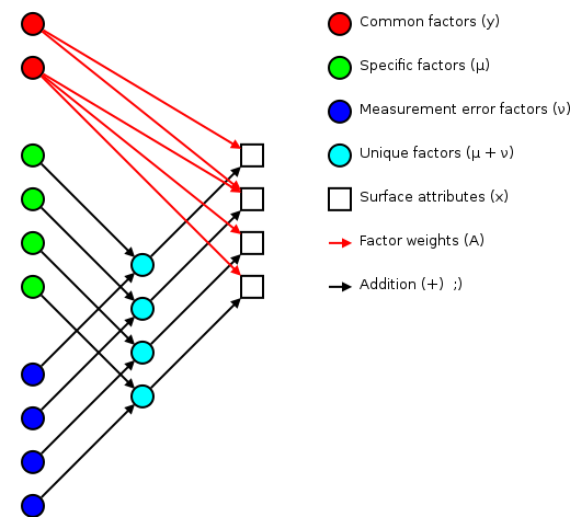Corresponding to the equation (Welling's eq. 1):

The independent random variables $y$ are distributed according to a Gaussian with zero mean and unit variance ${𝒢}_y[0,I]$ (zero mean because constant offsets are handled by $\mu$; unit variance becase scaling is handled by $A$). The independent random variables $\nu$ are distributed according to ${𝒢}_{\nu }[0,\Sigma ]$, with (Welling's eq. 2):

Because the only source of constant offset is $\mu$, we can calculate it by averaging out the random noise (Welling's eq. 6):

where $N$ is the number of measurements (survey responders) and $x_n$ is the response vector for the $n^{\text{th}}$ responder.

How do we find $A$ and $\Sigma$? This is the tricky bit, and there are a number of possible approaches. Welling suggests using expectation maximization (EM), and there's an excellent example of the procedure with a colorblind experimenter drawing colored balls in his EM notes (to test my understanding, I wrote color-ball.py).

To simplify calculations, Welling defines (before eq. 15):

which reduce the model to

After some manipulation Welling works out the maximizing updates (eq'ns 16 and 17):

The expectation values used in these updates are given by (Welling's eq'ns 12 and 13):

Survey analysis

Enough abstraction! Let's look at an example: survey results:

>>> import numpy
>>> scores = numpy.genfromtxt('Factor_analysis/survey.data', delimiter='\t')
>>> scores
array([[ 1.,  3.,  4.,  6.,  7.,  2.,  4.,  5.],
       [ 2.,  3.,  4.,  3.,  4.,  6.,  7.,  6.],
       [ 4.,  5.,  6.,  7.,  7.,  2.,  3.,  4.],
       [ 3.,  4.,  5.,  6.,  7.,  3.,  5.,  4.],
       [ 2.,  5.,  5.,  5.,  6.,  2.,  4.,  5.],
       [ 3.,  4.,  6.,  7.,  7.,  4.,  3.,  5.],
       [ 2.,  3.,  6.,  4.,  5.,  4.,  4.,  4.],
       [ 1.,  3.,  4.,  5.,  6.,  3.,  3.,  4.],
       [ 3.,  3.,  5.,  6.,  6.,  4.,  4.,  3.],
       [ 4.,  4.,  5.,  6.,  7.,  4.,  3.,  4.],
       [ 2.,  3.,  6.,  7.,  5.,  4.,  4.,  4.],
       [ 2.,  3.,  5.,  7.,  6.,  3.,  3.,  3.]])

scores[i,j] is the answer the ith respondent gave for the jth question. We're looking for underlying factors that can explain covariance between the different questions. Do the question answers ($x$) represent some underlying factors ($y$)? Let's start off by calculating $\mu$:

>>> def print_row(row):
...     print('  '.join('{: 0.2f}'.format(x) for x in row))
>>> mu = scores.mean(axis=0)
>>> print_row(mu)
 2.42   3.58   5.08   5.75   6.08   3.42   3.92   4.25

Next we need priors for $A$ and $\Sigma$. MDP has an implementation for Python, and their FANode uses a Gaussian random matrix for $A$ and the diagonal of the score covariance for $\Sigma$. They also use the score covariance to avoid repeated summations over $n$.

>>> import mdp
>>> def print_matrix(matrix):
...     for row in matrix:
...         print_row(row)
>>> fa = mdp.nodes.FANode(output_dim=3)
>>> numpy.random.seed(1)  # for consistend doctest results
>>> responder_scores = fa(scores)   # hidden factors for each responder
>>> print_matrix(responder_scores)
-1.92  -0.45   0.00
 0.67   1.97   1.96
 0.70   0.03  -2.00
 0.29   0.03  -0.60
-1.02   1.79  -1.43
 0.82   0.27  -0.23
-0.07  -0.08   0.82
-1.38  -0.27   0.48
 0.79  -1.17   0.50
 1.59  -0.30  -0.41
 0.01  -0.48   0.73
-0.46  -1.34   0.18
>>> print_row(fa.mu.flat)
 2.42   3.58   5.08   5.75   6.08   3.42   3.92   4.25
>>> fa.mu.flat == mu  # MDP agrees with our earlier calculation
array([ True,  True,  True,  True,  True,  True,  True,  True], dtype=bool)
>>> print_matrix(fa.A)  # factor weights for each question
 0.80  -0.06  -0.45
 0.17   0.30  -0.65
 0.34  -0.13  -0.25
 0.13  -0.73  -0.64
 0.02  -0.32  -0.70
 0.61   0.23   0.86
 0.08   0.63   0.59
-0.09   0.67   0.13
>>> print_row(fa.sigma)  # unique noise for each question
 0.04   0.02   0.38   0.55   0.30   0.05   0.48   0.21

Because the covariance is unaffected by the rotation $A\to AR$, the estimated weights $A$ and responder scores $y$ can be quite sensitive to the seed priors. The width $\Sigma$ of the unique noise $\nu$ is more robust, because $\Sigma$ is unaffected by rotations on $A$.

Nomenclature

$A_{\mathrm{ij}}$

The element from the $i^{\text{th}}$ row and $j^{\text{th}}$ column of a matrix $A$. For example here is a 2-by-3 matrix terms of components:

(8)$$A=\left(\begin{array}{ccc}{A}_{11}& A_{12}& A_{13}\\ A_{21}& A_{22}& A_{23}\end{array}\right)$$

$A^T$

The transpose of a matrix (or vector) $A$. $A_{\mathrm{ij}}^T=A_{\mathrm{ji}}$

$A^{-1}$

The inverse of a matrix $A$. $A^{-1}\dot{A}=1$

$\text{diag}[A]$

A matrix containing only the diagonal elements of $A$, with the off-diagonal values set to zero.

$E[f(x)]$

Expectation value for a function $f$ of a random variable $x$. If the probability density of $x$ is $p(x)$, then $E[f(x)]=\int dxp(x)f(x)$. For example, $E[p(x)]=1$.

$\mu$

The mean of a random variable $x$ is given by $\mu =E[x]$.

$\Sigma$

The covariance of a random variable $x$ is given by $\Sigma =E[(x-\mu )(x-\mu {)}^T]$. In the factor analysis model discussed above, $\Sigma$ is restricted to a diagonal matrix.

${𝒢}_x[\mu ,\Sigma ]$

A Gaussian probability density for the random variables $x$ with a mean $\mu$ and a covariance $\Sigma$.

(9)$${𝒢}_x[\mu ,\Sigma ]=\frac{1}{(2\pi {)}^{\frac{D}{2}}\sqrt{\det [\Sigma ]}}{e}^{-\frac{1}{2}(x-\mu {)}^T{\Sigma }^{-1}(x-\mu )}$$

$p(y\mid x)$

Probability of $y$ occurring given that $x$ occured. This is commonly used in Bayesian statistics.

$p(x,y)$

Probability of $y$ and $x$ occuring simultaneously (the joint density). $p(x,y)=p(x\mid y)p(y)$

Note: if you have trouble viewing some of the more obscure Unicode used in this post, you might want to install the STIX fonts.

Available in a git repository.
Repository: catalyst-swc
Browsable repository: catalyst-swc
Author: W. Trevor King

Catalyst is a release-building tool for Gentoo. If you use Gentoo and want to roll your own live CD or bootable USB drive, this is the way to go. As I've been wrapping my head around catalyst, I've been pushing my notes upstream. This post builds on those notes to discuss the construction of a bootable ISO for Software Carpentry boot camps.

Getting a patched up catalyst

Catalyst has been around for a while, but the user base has been fairly small. If you try to do something that Gentoo's Release Engineering team doesn't do on a regular basis, built in catalyst support can be spotty. There's been a fair amount of patch submissions an gentoo-catalyst@ recently, but patch acceptance can be slow. For the SWC ISO, I applied versions of the following patches (or patch series) to 37540ff:

• chmod +x all sh scripts so they can run from the git checkout
• livecdfs-update.sh: Set XSESSION in /etc/env.d/90xsession
• Fix livecdfs-update.sh startx handling

Configuring catalyst

The easiest way to run catalyst from a Git checkout is to setup a local config file. I didn't have enough hard drive space on my local system (~16 GB) for this build, so I set things up in a temporary directory on an external hard drive:

$ cat catalyst.conf | grep -v '^#\|^$'
digests="md5 sha1 sha512 whirlpool"
contents="auto"
distdir="/usr/portage/distfiles"
envscript="/etc/catalyst/catalystrc"
hash_function="crc32"
options="autoresume kerncache pkgcache seedcache snapcache"
portdir="/usr/portage"
sharedir="/home/wking/src/catalyst"
snapshot_cache="/mnt/d/tmp/catalyst/snapshot_cache"
storedir="/mnt/d/tmp/catalyst"

I used the default values for everything except sharedir, snapshot_cache, and storedir. Then I cloned the catalyst-swc repository into /mnt/d/tmp/catalyst.

Portage snapshot and a seed stage

Take a snapshot of the current Portage tree:

# catalyst -c catalyst.conf --snapshot 20130208

Download a seed stage3 from a Gentoo mirror:

# wget -O /mnt/d/tmp/catalyst/builds/default/stage3-i686-20121213.tar.bz2 \
>   http://distfiles.gentoo.org/releases/x86/current-stage3/stage3-i686-20121213.tar.bz2

Building the live CD

# catalyst -c catalyst.conf -f /mnt/d/tmp/catalyst/spec/default-stage1-i686-2013.1.spec
# catalyst -c catalyst.conf -f /mnt/d/tmp/catalyst/spec/default-stage2-i686-2013.1.spec
# catalyst -c catalyst.conf -f /mnt/d/tmp/catalyst/spec/default-stage3-i686-2013.1.spec
# catalyst -c catalyst.conf -f /mnt/d/tmp/catalyst/spec/default-livecd-stage1-i686-2013.1.spec
# catalyst -c catalyst.conf -f /mnt/d/tmp/catalyst/spec/default-livecd-stage2-i686-2013.1.spec

isohybrid

To make the ISO bootable from a USB drive, I used isohybrid:

# cp swc-x86.iso swc-x86-isohybrid.iso
# isohybrid iso-x86-isohybrid.iso

You can install the resulting ISO on a USB drive with:

# dd if=iso-x86-isohybrid.iso of=/dev/sdX

replacing replacing X with the appropriate drive letter for your USB drive.

With versions of catalyst after d1c2ba9, the isohybrid call is built into catalysts ISO construction.

SymPy is a Python library for symbolic mathematics. To give you a feel for how it works, lets extrapolate the extremum location for $f(x)$ given a quadratic model:

and three known values:

Rephrase as a matrix equation:

So the solutions for $A$, $B$, and $C$ are:

Now that we've found the model parameters, we need to find the $x$ coordinate of the extremum.

which is zero when

Here's the solution in SymPy:

>>> from sympy import Symbol, Matrix, factor, expand, pprint, preview
>>> a = Symbol('a')
>>> b = Symbol('b')
>>> c = Symbol('c')
>>> fa = Symbol('fa')
>>> fb = Symbol('fb')
>>> fc = Symbol('fc')
>>> M = Matrix([[a**2, a, 1], [b**2, b, 1], [c**2, c, 1]])
>>> F = Matrix([[fa],[fb],[fc]])
>>> ABC = M.inv() * F
>>> A = ABC[0,0]
>>> B = ABC[1,0]
>>> x = -B/(2*A)
>>> x = factor(expand(x))
>>> pprint(x)
 2       2       2       2       2       2   
a *fb - a *fc - b *fa + b *fc + c *fa - c *fb
---------------------------------------------
 2*(a*fb - a*fc - b*fa + b*fc + c*fa - c*fb) 
>>> preview(x, viewer='pqiv')

Where pqiv is the executable for pqiv, my preferred image viewer. With a bit of additional factoring, that is:

Since I love both teaching and open source development, I suppose it was only a matter of time before I attempted a survey of open source text books. Here are my notes on the projects I've come across so far:

Light and Matter

The Light and Matter series is a set of six texts by Benjamin Crowell at Fullerton College in California. The series is aimed at the High School and Biology (i.e. low calc) audience. The source is distributed in LaTeX and versioned in Git. I love this guy!

Crowell also runs a book review site The Assayer, which reviews free books.

Radically Modern Introductory Physics

Radically Modern Introductory Physics is David J. Raymond's modern-physics-based approach to introductory physics. He posts the LaTeX source, but it does not seem to be version controlled.

Calculus Based Physics

Calculus Based Physics, by Jeffrey W. Schnick at St. Anselm in New Hampshire. It is under the Creative Commons Attribution-ShareAlike 3.0 License, and the sources are free to alter. However, there is no official version control, and the sources are in MS Word format :(. On the other hand, I wholeheartedly agree with all the objectives Schnick lists in his motivational note.

Textbook Revolution

Calculus Based Physics' Schnick linked to Textbook Revolution, which immediately gave off good tech vibes with an IRC node (#textbookrevolution). The site is basically a wiki with a browsable list of pointers to open textbooks. The list isn't huge, but it does prominently display copyright information, which makes it easier to separate the wheat from the chaff.

College Open Textbooks

College Open Textbooks provides another registry of open textbooks with clearly listed license information. They're funded by The William and Flora Hewlett Foundation (of NPR underwriting fame).

MERLOT's Open Textbook Initiative

The Multimedia Educational Resource for Learning and Online Teaching (MERLOT) is a California-based project that assembles educational resources. They have a large collection of open textbooks in a variety of fields. The Light and Matter series is well represented. Unfortunately, many of the texts seem to be "free as in beer" not "free as in freedom".

Open Access Textbooks

The Open Access Textbooks project is run by a number of Florida-based groups and funded by the U.S. Department of Education. However, I have grave doubts about any open source project that opens their project discussion with

Numerous issues that impact open textbook implementation (such as creating sustainable review processes and institutional reward structures) have yet to be resolved. The ability to financially sustain a large scale open textbook effort is also in question.

There are zounds of academics with enough knowledge and invested interest in developing an open source textbook. The resources (computers and personal websites) are generally already provided by academic institutions. Just pick a framework (LaTeX, HTML, ...), put the whole thing in Git, and start hacking. The community will take it from there.

Anyhow, everything I've read about this project smells like a bunch of bureaucrat's churning out sound bytes.

ArXiv

Finally, there are a number of textbooks on arXiv. For example, Siegel's Introduction to string field theory and Fields are posted source and all. The source will probably be good quality, but the licensing information may be unclear.

Available in a git repository.
Repository: parallel_computing
Browsable repository: parallel_computing
Author: W. Trevor King

In contrast to my course website project, which is mostly about constructing a framework for automatically compiling and installing LaTeX problem sets, Prof. Vallières' Parallel Computing course is basically an online textbook with a large amount of example software. In order to balance between to Prof. Vallières' original and my own aesthetic, I rolled a new solution from scratch. See my version of his Fall 2010 page for a live example.

Differences from my course website project:

• No PHP, since there is no dynamic content that cannot be handled with SSI.
• Less installation machinery. Only a few build/cleanup scripts to avoid versioning really tedious bits. The repository is designed to be dropped into your ~/public_html/ whole, while the course website project is designed to rsync the built components up as they go live.
• Less LaTeX, more XHTML. It's easier to edit XHTML than it is to exit and compile LaTeX, and PDFs are large and annoying. As a computing class, there are fewer graphics than there are in an intro-physics class, so the extra power of LaTeX is not as useful.

Available in a git repository.
Repository: course
Browsable repository: course
Author: W. Trevor King

Over a few years as a TA for assorted introductory physics classes, I've assembled a nice website framework with lots of problems using my LaTeX problempack package, along with some handy Makefiles, a bit of php, and SSI.

The result is the course package, which should make it very easy to whip up a course website, homeworks, etc. for an introductory mechanics or E&M class (431 problems implemented as of June 2012). With a bit of work to write up problems, the framework could easily be extended to other subjects.

The idea is that a course website consists of a small, static HTML framework, and a bunch of content that is gradually filled in as the semester/quarter progresses. I've put the HTML framework in the html/ directory, along with some of the write-once-per-course content (e.g. Prof & TA info). See html/README for more information on the layout of the HTML.

The rest of the directories contain the code for compiling material that is deployed as the course progresses. The announcements/ directory contains the atom feed for the course, and possibly a list of email addresses of people who would like to (or should) be notified when new announcements are posted. The latex/ directory contains LaTeX source for the course documents for which it is available, and the pdf/ directory contains PDFs for which no other source is available (e.g. scans, or PDFs sent in by Profs or TAs who neglected to include their source code).

Note that because this framework assumes the HTML content will be relatively static, it may not be appropriate for courses with large amounts of textbook-style content, which will undergo more frequent revision. It may also be excessive for courses that need less compiled content. For an example of another framework, see my branch of Prof. Vallières' Parallel Computing website.

Available in a git repository.
Repository: problempack
Browsable repository: problempack
Author: W. Trevor King

I've put together a LaTeX package problempack to make it easier to write up problem sets with solutions for the classes I TA.

problempack.sty

The package takes care of a few details:

• Make it easy to compile one pdf with only the problems and another pdf with problems and solutions.
• Define nicely typeset environments for automatically or manually numbered problems.
• Save retyping a few of the parameters (course title, class title, etc), that show up in the note title and also need to go out to pdftitle and pdfsubject.
• Change the page layout to minimize margins (saves paper on printing).
• Set the spacing between problems (e.g. to tweak output to a single page, versions >= 0.2).
• Add section level entries to the table-of-contents and hyperref bookmarks (versions >= 0.3).

The basic idea is to make it easy to write up notes. Just install problempack.sty in your texmf tree, and then use it like I do in the example included in the package. The example produces a simple problem set (probs.pdf) and solution notes (sols.pdf).

For a real world example, look at my Phys 102 notes with and without solutions (source). Other notes produced in this fashion: Phys201 winter 2009, Phys201 spring 2009, and Phys102 summer 2009.

wtk_cmmds.sty

A related package that defines some useful physics macros (\U, \E, \dg, \vect, \ihat, ...) is my wtk_cmmds.sty. This used to be a part of problempack.sty, but the commands are less general, so I split them out into their own package.

wtk_format.sty

The final package in the problempack repository is wtk_format.sty, which adjusts the default LaTeX margins to pack more content into a single page.

I've had a few students confused by this sort of "zooming and chunking" approach to analyzing functions specifically, and technical problems in general, so I'll pass the link on in case you're interested. Curtesy of Charles Wells.