Theory pages.

RSS Atom

I've been trying to wrap my head around factor analysis as a theory for designing and understanding test and survey results. This has turned out to be another one of those fields where the going has been a bit rough. I think the key factors in making these older topics difficult are:

“Everybody knows this, so we don't need to write up the details.”
“Hey, I can do better than Bob if I just tweak this knob…”
“I'll just publish this seminal paper behind a paywall…”

The resulting discussion ends up being overly complicated, and it's hard for newcomers to decide if people using similar terminology are in fact talking about the same thing.

Some of the better open sources for background has been Tucker and MacCallum's “Exploratory Factor Analysis” manuscript and Max Welling's notes. I'll use Welling's terminology for this discussion.

The basic idea of factor analsys is to model $d$ measurable attributes as generated by $k < d$ common factors and $d$ unique factors. With $n = 4$ and $k = 2$ , you get something like:

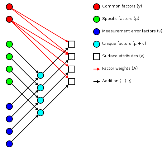Relationships between factors and measured attributes (adapted from Tucker and MacCallum's Figure 1.2)

Corresponding to the equation (Welling's eq. 1):

(1)

x = A y + μ + ν

The independent random variables $y$ are distributed according to a Gaussian with zero mean and unit variance $𝒢_{y} [0, I]$ (zero mean because constant offsets are handled by $μ$ ; unit variance because scaling is handled by $A$ ). The independent random variables $ν$ are distributed according to $𝒢_{ν} [0, Σ]$ , with (Welling's eq. 2):

(2)

Σ \equiv diag [σ_{1}^{2}, \dots, σ_{d}^{2}]

The matrix $A$ (linking common factors with measured attributes $x) is refered to as the factor weights or factor loadings . Because the only source of constant offset is$ \mathbf{\mu} $, we can calculate it by averaging out the random noise (Welling' s eq . 6) : Unknown character div class = Unknown character numberedEq Unknown character Unknown character Unknown character span Unknown character (3) Unknown character / span Unknown character$ $μ = \frac{1}{N} \sum_{n = 1}^{N} x_{n}$ $Unknown character / div Unknown character where$ N $is the number of measurements (survey responders) and$ \mathbf{x}n $is the response vector for the$ n^\text{th} $responder . How do we find$ \mathbf{A} $and$ \mathbf{\Sigma} $? This is the tricky bit, and there are a number of possible approaches . Welling suggests using expectation maximization (EM), and there' s an excellent example of the procedure with a colorblind experimenter drawing colored balls in his [EM notes] [EM] (to test my understanding, I wrote Unknown character a href = Unknown character . . / . . / posts / {Factor}_{analysis} / color - ball . py Unknown character Unknown character color - ball . py Unknown character / a Unknown character) . To simplify calculations, Welling defines (before eq . 15) : Unknown character div class = Unknown character numberedEq Unknown character Unknown character Unknown character span Unknown character (4) Unknown character / span Unknown character$ $\begin{aligned} A' & \equiv [A, μ] \\ y' & \equiv [y^{T}, 1]^{T} \end{aligned}$ $Unknown character / div Unknown character which reduce the model to Unknown character div class = Unknown character numberedEq Unknown character Unknown character Unknown character span Unknown character (5) Unknown character / span Unknown character$ $x = A' y' + ν$ $Unknown character / div Unknown character After some manipulation Welling works out the maximizing updates (eq' ns 16 and 17) : Unknown character div class = Unknown character numberedEq Unknown character Unknown character Unknown character span Unknown character (6) Unknown character / span Unknown character$ $\begin{aligned} A'^{new} & = (\sum_{n = 1}^{N} x_{n} E [y' ∣ x_{n}]^{T}) {(\sum_{n = 1}^{N} x_{n} E [y' y'^{T} ∣ x_{n}])}^{- 1} \\ Σ^{new} & = \frac{1}{N} \sum_{n = 1}^{N} diag [x_{n} x_{n}^{T} - A'^{new} E [y' ∣ x_{n}] x_{n}^{T}] \end{aligned}$ $Unknown character / div Unknown character The expectation values used in these updates are given by (Welling' s eq' ns 12 and 13) : Unknown character div class = Unknown character numberedEq Unknown character Unknown character Unknown character span Unknown character (7) Unknown character / span Unknown character$ $\begin{aligned} E [y ∣ x_{n}] & = A^{T} (A A^{T} + Σ)^{- 1} (x_{n} - μ) \\ E [y y^{T} ∣ x_{n}] & = I - A^{T} (A A^{T} + Σ)^{- 1} A + E [y ∣ x_{n}] E [y ∣ x_{n}]^{T} \end{aligned}$ $Unknown character / div Unknown character Survey analysis = = = = = = = = = = = = = = = Enough abstraction! Let' s look at an example : [survey results] [survey] : Unknown character Unknown character Unknown character import numpy Unknown character Unknown character Unknown character scores = numpy . genfromtxt (' {Factor}_{analysis} / survey . data', delimiter =' t') Unknown character Unknown character Unknown character scores array ([[1 ., 3 ., 4 ., 6 ., 7 ., 2 ., 4 ., 5 .], [2 ., 3 ., 4 ., 3 ., 4 ., 6 ., 7 ., 6 .], [4 ., 5 ., 6 ., 7 ., 7 ., 2 ., 3 ., 4 .], [3 ., 4 ., 5 ., 6 ., 7 ., 3 ., 5 ., 4 .], [2 ., 5 ., 5 ., 5 ., 6 ., 2 ., 4 ., 5 .], [3 ., 4 ., 6 ., 7 ., 7 ., 4 ., 3 ., 5 .], [2 ., 3 ., 6 ., 4 ., 5 ., 4 ., 4 ., 4 .], [1 ., 3 ., 4 ., 5 ., 6 ., 3 ., 3 ., 4 .], [3 ., 3 ., 5 ., 6 ., 6 ., 4 ., 4 ., 3 .], [4 ., 4 ., 5 ., 6 ., 7 ., 4 ., 3 ., 4 .], [2 ., 3 ., 6 ., 7 ., 5 ., 4 ., 4 ., 4 .], [2 ., 3 ., 5 ., 7 ., 6 ., 3 ., 3 ., 3 .]]) </mo><mi>scores</mi><mo stretchy="false">[</mo><mi>i</mi><mo>,</mo><mi>j</mi><mo stretchy="false">]</mo><mo> is the answer the </mo><mi>i</mi><mo> th respondent gave for the </mo><mi>j</mi><mo> th question . We' re looking for underlying factors that can explain covariance between the different questions . Do the question answers ($ \mathbf{x} $) represent some underlying factors ($ \mathbf{y} $) ? Let' s start off by calculating$ \mathbf{\mu} $: Unknown character Unknown character Unknown character def {print}_{row} (row) : . . . print ('' . join (' : 0.2 f' . format (x) for x in row)) Unknown character Unknown character Unknown character mu = scores . mean (axis = 0) Unknown character Unknown character Unknown character {print}_{row} (mu) 2.42 3.58 5.08 5.75 6.08 3.42 3.92 4.25 Next we need priors for$ \mathbf{A} $and$ \mathbf{\Sigma} $. Unknown character span class = Unknown character createlink Unknown character Unknown character MDP Unknown character / span Unknown character has an implementation for Unknown character a href = Unknown character . . / . . / posts / Python / Unknown character Unknown character Python Unknown character / a Unknown character, and their [FANode] [] uses a Gaussian random matrix for$ \mathbf{A} $and the diagonal of the score covariance for$ \mathbf{\Sigma} $. They also use the score covariance to avoid repeated summations over$ n $. Unknown character Unknown character Unknown character import mdp Unknown character Unknown character Unknown character def {print}_{matrix} (matrix) : . . . for row in matrix : . . . {print}_{row} (row) Unknown character Unknown character Unknown character fa = mdp . nodes . FANode ({output}_{\dim} = 3) Unknown character Unknown character Unknown character numpy . random . seed (1) # for consistend doctest results Unknown character Unknown character Unknown character {responder}_{scores} = fa (scores) # common factors for each responder Unknown character Unknown character Unknown character {print}_{matrix} ({responder}_{scores}) - 1.92 - 0.45 0.00 0.67 1.97 1.96 0.70 0.03 - 2.00 0.29 0.03 - 0.60 - 1.02 1.79 - 1.43 0.82 0.27 - 0.23 - 0.07 - 0.08 0.82 - 1.38 - 0.27 0.48 0.79 - 1.17 0.50 1.59 - 0.30 - 0.41 0.01 - 0.48 0.73 - 0.46 - 1.34 0.18 Unknown character Unknown character Unknown character {print}_{row} (fa . mu . flat) 2.42 3.58 5.08 5.75 6.08 3.42 3.92 4.25 Unknown character Unknown character Unknown character fa . mu . flat = = mu # MDP agrees with our earlier calculation array ([True, True, True, True, True, True, True, True], dtype = bool) Unknown character Unknown character Unknown character {print}_{matrix} (fa . A) # factor weights for each question 0.80 - 0.06 - 0.45 0.17 0.30 - 0.65 0.34 - 0.13 - 0.25 0.13 - 0.73 - 0.64 0.02 - 0.32 - 0.70 0.61 0.23 0.86 0.08 0.63 0.59 - 0.09 0.67 0.13 Unknown character Unknown character Unknown character {print}_{row} (fa . sigma) # unique noise for each question 0.04 0.02 0.38 0.55 0.30 0.05 0.48 0.21 Because the covariance is unaffected by the rotation$ \mathbf{A}\rightarrow\mathbf{A}\mathbf{R} $, the estimated weights$ \mathbf{A} $and responder scores$ \mathbf{y} $can be quite sensitive to the seed priors . The width$ \mathbf{\Sigma} $of the unique noise$ \mathbf{\nu} $is more robust, because$ \mathbf{\Sigma} $is unaffected by rotations on$ \mathbf{A} $. Related tidbits = = = = = = = = = = = = = = = Communality - - - - - - - - - - - The [communality] []$ hi^2 $of the$ i^\text{th} $measured attribute$ x_i $is the fraction of variance in the measured attribute which is explained by the set of common factors . Because the common factors$ \mathbf{y} $have unit variance, the communality is given by : Unknown character div class = Unknown character numberedEq Unknown character Unknown character Unknown character span Unknown character (8) Unknown character / span Unknown character$ $h_{i} = \frac{\sum_{j = 1}^{k} A_{ij}^{2}}{\sum_{j = 1}^{k} A_{ij}^{2} + σ_{1}^{2}}$ $Unknown character / div Unknown character Unknown character Unknown character Unknown character {factor}_{variance} = numpy . array ([sum (row 2) for row in fa . A]) Unknown character Unknown character Unknown character h = numpy . array (. . . [var / (var + sig) for var, sig in zip ({factor}_{variance}, fa . sigma)]) Unknown character Unknown character Unknown character {print}_{row} (h) 0.95 0.97 0.34 0.64 0.66 0.96 0.61 0.69 There may be some scaling issues in the communality due to deviations between the estimated$ \mathbf{A} $and Σ$ and the variations contained in the measured scores (why?):

>>> print_row(factor_variance + fa.sigma)
 0.89   0.56   0.57   1.51   0.89   1.21   1.23   0.69
>>> print_row(scores.var(axis=0, ddof=1))  # total variance for each question
 0.99   0.63   0.63   1.66   0.99   1.36   1.36   0.75

The proportion of total variation explained by the common factors is given by:

(9)

\frac{\sum_{i = 1}^{k} h_{i}}{}

Varimax rotation

As mentioned earlier, factor analysis generated loadings $A$ that are unique up to an arbitrary rotation $R$ (as you'd expect for a $k$ -dimensional Gaussian ball of factors $y$ ). A number of of schemes have been proposed to simplify the initial loadings by rotating $A$ to reduce off-diagonal terms. One of the more popular approaches is Henry Kaiser's varimax rotation (unfortunately, I don't have access to either his thesis or the subsequent paper). I did find (via Wikipedia) Trevor Park's notes which have been very useful.

The idea is to iterate rotations to maximize the raw varimax criterion (Park's eq. 1):

(10)

V (A) = \sum_{j = 1}^{k} (\frac{1}{d} \sum_{i = 1}^{d} A_{ij}^{4} - {(\frac{1}{d} \sum_{i = 1}^{d} A_{ij}^{4})}^{2})

Rather than computing a $k$ -dimensional rotation in one sweep, we'll iterate through 2-dimensional rotations (on successive column pairs) until convergence. For a particular column pair $(p, q)$ , the rotation matrix $R^{*}$ is the usual rotation matrix:

(11)

R^{*} = (\begin{matrix} \cos (ϕ^{*}) & - \sin (ϕ^{*}) \\ \sin (ϕ^{*}) & \cos (ϕ^{*}) \end{matrix})

where the optimum rotation angle $ϕ^{*}$ is (Park's eq. 3):

(12)

ϕ^{*} = \frac{1}{4} ∠ (\frac{1}{d} \sum_{j = 1}^{d} {(A_{jp} + {iA}_{jq})}^{4} - {(\frac{1}{d} \sum_{j = 1}^{d} {(A_{jp} + {iA}_{jq})}^{2})}^{2})

where $i \equiv \sqrt{- 1}$ .

Nomenclature

$A_{ij}$: The element from the $i^{th}$ row and $j^{th}$ column of a matrix $A$ . For example here is a 2-by-3 matrix terms of components:
(13) $A = (\begin{matrix} A_{11} & A_{12} & A_{13} \\ A_{21} & A_{22} & A_{23} \end{matrix})$
$A^{T}$: The transpose of a matrix (or vector) $A$ . $A_{ij}^{T} = A_{ji}$
$A^{- 1}$: The inverse of a matrix $A$ . $A^{- 1} \dot{A} = 1$
$diag [A]$: A matrix containing only the diagonal elements of $A$ , with the off-diagonal values set to zero.
$E [f (x)]$: Expectation value for a function $f$ of a random variable $x$ . If the probability density of $x$ is $p (x)$ , then $E [f (x)] = \int d x p (x) f (x)$ . For example, $E [p (x)] = 1$ .
$μ$: The mean of a random variable $x$ is given by $μ = E [x]$ .
$Σ$: The covariance of a random variable $x$ is given by $Σ = E [(x - μ) (x - μ)^{T}]$ . In the factor analysis model discussed above, $Σ$ is restricted to a diagonal matrix.
$𝒢_{x} [μ, Σ]$: A Gaussian probability density for the random variables $x$ with a mean $μ$ and a covariance $Σ$ .
(14) $𝒢_{x} [μ, Σ] = \frac{1}{(2 π)^{\frac{D}{2}} \sqrt{\det [Σ]}} e^{- \frac{1}{2} (x - μ)^{T} Σ^{- 1} (x - μ)}$
$p (y ∣ x)$: Probability of $y$ occurring given that $x$ occured. This is commonly used in Bayesian statistics.
$p (x, y)$: Probability of $y$ and $x$ occuring simultaneously (the joint density). $p (x, y) = p (x ∣ y) p (y)$
$∠ (z)$: The angle of $z$ in the complex plane. $∠ ({re}^{i θ}) = θ$ .

Note: if you have trouble viewing some of the more obscure Unicode used in this post, you might want to install the STIX fonts.

I've been spending some time comparing my force spectroscopy data with Marisa's, and the main problem has been normalizing the data collected using different systems. Marisa runs experiments using some home-grown LabVIEW software, which saves the data in IGOR binary wave (IBW) files. From my point of view, this is not the best approach, but it has been stable over the time we've been running experiments.

I run my own experiments using my own code based on pyafm, saving the data in HDF5 files. I think this approach is much stronger, but it has been a bit of a moving target, and I've spent a good deal of my time working on the framework instead of running experiments.

Both approaches save the digitized voltages that we read/write during an experiment, but other constants and calibration terms are not always recorded. My pyafm-based software has been gradually getting better in this regard, especially since I moved to h5config-based initialization. Anyhow, here's a quick runthough of all the important terms.

For the TL;DR crowd, crunch.py is my Python module that crunches your input and prints out all the intermediate constants discussed below. To use it on your own data, you'll probably have to tweak the bits that read in the data to use your own format.

Calibrating the piezo

Calibration grid

We control the surface-tip distance by driving a piezo tube. We want to know the correspondence between the driving voltage and the piezo position, so we calibrate the piezo by imaging a sample with square pits of a known depth.

In this trace, I swept the $x$ position across most of the range of my 16-bit DAC. For each $x$ position, I adjusted the $z$ position until the measured cantilever deflection $d$ crossed a setpoint. This gives the $z$ voltage required to reach the surface as a function of $x$ . You can see the 200 nm deep square pits, as well as a reasonable amount of $x$ / $z$ crosstalk.

Sometimes grid calibrations are even less convincing than the example shown above. For example, I have traces with odd shoulders on the sides of the pits:

This is one of the better piezo calibration images I aquired for the piezo used in the pull below, so I'll use numbers from the funky imaging for the remainder of this analysis. This piezo has less $x$ / $y$ range than the one used to measure the first calibration trace, which is why I was unable to aquire a full pit (or pits).

The calibration constant $α_{z}$ is the number of $z$ bits per depth meter:

(1)

α_{z} = \frac{grid piezo bits}{grid depth} = \frac{2779 \pm 87 bits}{200 nm} = (1.39 \pm 0.04) \cdot 10^{10} bits/m .

Related conversion factors are

(2)

\begin{aligned} γ_{z} & = \frac{piezo volts}{piezo bits} = \frac{20 piezo volts}{output volts} \cdot \frac{10 output volts}{2^{15} piezo bits} = 6.10 \cdot 10^{- 3} V/bit \\ σ_{z} & = \frac{grid piezo volts}{grid depth} = γ_{z} α_{z} = 8.48 \cdot 10^{7} V/m . \end{aligned}

This is roughly in the ballpark of our piezo (serial number 2253E) which is spec'd at 8.96 nm/V along the $z$ axis, which comes out to $1.12 \cdot 10^{8}$ V/m.

Laser interference

Another way to ballpark a piezo calibration that is much closer to a force spectroscopy pull is to use the laser interference pattern as a standard length. The laser for our microscope has a wavelength of 670 nm. We'll assume a geometric gain of

(3)

g_{λ} = \frac{increased laser path}{piezo displacement} \approx 2 .

Measuring the length of an interference wave in bits then gives a standard equivalent to the known-depth pits of the calibration grid.

(4)

\begin{aligned} α_{z} & = \frac{interference piezo bits}{interference depth} = \frac{g_{λ}}{λ} \cdot interference piezo bits \\ = \frac{2}{670 \cdot 10^{- 9} m} \cdot (28935 - 23721) bits = 1.56 \cdot 10^{10} bits/m . \end{aligned}

The other piezo calibration parameters are found exactly as in the calibration grid case.

(5)

σ_{z} = γ_{z} α_{z} = 9.52 \cdot 10^{7} V/m .

which is fairly close to both the spec'd value and grid calibration values.

Calibrating the photodiode

During experiments, we measure cantilever deflection via the top and bottom segments of a photodiode. We need to convert this deflection voltage into a deflection distance, so we'll use the already-calibrated piezo. When the tip is in contact with the surface, we can move the surface a known distance (using the piezo) and record the change in deflection.

The calibration constant $α_{d}$ is the number of diode bits per piezo bit.

(6)

α_{d} = \frac{bump diode bits}{bump piezo bits} = 2.24 diode bits/piezo bits .

Related conversion factors are

(7)

\begin{aligned} γ_{d} & = \frac{diode volts}{diode bits} = \frac{10 input volts}{2^{15} diode bits} \cdot \frac{diode volts}{1 input volts} = 3.05 \cdot 10^{- 4} V/bit \\ σ_{d} & = \frac{bump diode volts}{bump tip position} = γ_{d} α_{d} α_{z} = 9.52 \cdot 10^{6} V/m . \end{aligned}

Calibrating the cantilever spring constant

To convert cantilever tip deflection to force, we need to know the spring constant of the cantilever. After bumping the surface, we move away from the surface and measure the cantilever's thermal vibration. We use the vibration data to calculate the spring constant using the equipartition theorem.

The deflection variance $⟨ d^{2} ⟩$ is measured in frequency space, where the power spectral density (PSD) is fitted to the expected PSD of a damped harmonic oscillator.

(8)

\begin{aligned} {PSD}_{f} & = \frac{G_{1 f}}{(f_{0}^{2} - f^{2})^{2} + β_{f}^{2} f^{2}} \\ ⟨ d^{2} ⟩ & = \frac{π G_{1 f}}{2 β_{f} f_{0}^{2}} \\ κ & = \frac{2 β_{f} f_{0}^{2}}{π G_{1 f}} (α_{d} α_{z})^{2} k_{B} T = \frac{2 \cdot (4.17 \cdot 10^{3} Hz) \cdot (8.14 \cdot 10^{3} Hz)^{2}}{π \cdot 3.10 \cdot 10^{13} {bit}^{2} \cdot {Hz}^{3}} \cdot (2.24 \cdot 1.39 \cdot 10^{10} bit/m)^{2} \cdot (1.38 \cdot 10^{- 23} J/K) \cdot (294 K) = 22.4 \cdot 10^{- 3} N/m \end{aligned}

Analyzing a velocity-clamp pull

The raw data from a velocity-clamp pull is an array of output voltages used to sweep the piezo (moving the surface away from the cantilever tip) and an array of input voltages from the photodiode (measuring cantilever deflection). There are a number of interesting questions you can ask about such data, so I'll break this up into a few steps. Lets call the raw piezo data (in bits) $α_{v}$ , with the contact-kink located at $α_{v 0}$ . Call the raw deflection data (also in bits) $α_{F}$ , with the contact-kink located at $α_{F 0}$ .

Piezo displacement

Using the piezo calibration parameters, we can calculate the raw piezo position using

(9)

z_{piezo} = \frac{α_{v} - α_{v 0}}{α_{z}},

measured in meters.

Surface contact region

During the initial portion of a velocity clamp pull, the cantilever tip is still in contact with the surface. This allows you to repeat the photodiode calibration, avoiding problems due to drift in laser alignment or other geometric issues. This gives a new set of diode calibration parameters $α_{d}'$ and $σ_{d}'$ (it is unlikely that $γ_{d}$ has changed, but it's easy to rework the following arguments to include $γ_{d}'$ if you feel that it might have changed).

Tension

We can use the new photodiode calibration and the cantilever's spring constant to calculate the force from the Hookean cantilever:

(10)

F = \frac{α_{F} - α_{F 0}}{α_{d}' α_{z}} \cdot κ = (α_{F} - α_{F 0}) \cdot \frac{2 β_{f} f_{0}^{2}}{π G_{1 f}} \cdot \frac{α_{d}^{2} α_{z}}{α_{d}'} \cdot k_{B} T .

Protein extension

As the piezo pulls on the cantilever/protein system, some of the increased extension is due to protein extension and the rest is due to cantilever extension. We can use Hooke's law to remove the cantilever extension, leaving only protein extension:

(11)

z_{protein} = z_{piezo} - \frac{F}{κ} = \frac{1}{α_{z}} (α_{v} - α_{v 0} - \frac{α_{F} - α_{F 0}}{α_{d}'})

Contour-space

In order to confirm the piezo calibration, we look at changes in the unfolded contour length due to domain unfolding ( $Δ L$ ). There have been a number of studies of titin I27, starting with Carrion-Vazquez et al., that show an contour length increase of 28.1 ± 0.17 nm. Rather than fitting each loading region with a worm-like chain (WLC) or other polymer model, it is easier to calculate $Δ L$ by converting the abscissa to contour-length space (following Puchner et al.). While the WLC is commonly used, Puchner gets better fits using the freely rotating chain (FRC) model.

In crunch.py, I use either Bustamante's formula (WLC) or Livadaru's equation 49 (FRC) to calculate the contour length of a particular force/distance pair.

As you can see from the figure, my curves are spaced a bit too far appart. Because the contour length depends $F$ as well as $z_{protein}$ , it depends on the cantilever calibration (via $β_{f}$ , $f_{0}$ , $G_{1 f}$ and $α_{d}$ ) as well as the piezo calibration (via $α_{z}$ ). This makes adjusting calibration parameters in an attempt to match your $Δ L$ with previously determined values a bit awkward. However, it is likely that my cantilever calibration is too blame. If we use the value of $α_{z}$ from the interference measurement we get

Which is still a bit too wide, but is much closer.

Velocity clamp force spectroscopy pulls are often fit to polymer models such as the worm-like chain (WLC). However, Puchner et al. had the bright idea that, rather than fitting each loading region with a polymer model, it is easier to calculate the change in contour length by converting the abscissa to contour-length space. While the WLC is commonly used, Puchner gets better fits using the freely rotating chain (FRC) model.

Computing force-extension curves for either the WLC or FJC is complicated, and it is common to use interpolation formulas to estimate the curves. For the WLC, we use Bustamante's formula:

(1)

F_{WLC} (x) = \frac{k_{B} T}{p} [\frac{1}{4} (\frac{1}{{(1 - \frac{x}{L})}^{2}} - 1) + \frac{x}{L}]

For the FRC, Puchner uses Livadaru's equation 46.

(2)

\frac{R_{z}}{L} \approx {\begin{array}{ll} \frac{fa}{3 k_{B} T} & for \frac{fb}{k_{B} T} < \frac{b}{l} \\ 1 - {(\frac{fl}{4 k_{B} T})}^{- \frac{1}{2}} & for \frac{b}{l} < \frac{fb}{k_{B} T} < \frac{l}{b} \\ 1 - {(\frac{fb}{{ck}_{B} T})}^{- 1} & for \frac{l}{b} < \frac{fb}{k_{B} T} \end{array} .

Unfortunately, there are two typos in Livadaru's equation 46. It should read (confirmed by private communication with Roland Netz).

(3)

\frac{R_{z}}{L} \approx {\begin{array}{ll} \frac{fa}{3 k_{B} T} & for \frac{fb}{k_{B} T} < \frac{b}{l} \\ 1 - {(\frac{4 fl}{k_{B} T})}^{- \frac{1}{2}} & for \frac{b}{l} < \frac{fb}{k_{B} T} < \frac{l}{b} \\ 1 - {(\frac{cfb}{k_{B} T})}^{- 1} & for \frac{l}{b} < \frac{fb}{k_{B} T} \end{array} .

Regardless of the form of Livadaru's equation 46, the suggested FRC interpolation formula is Livadaru's equation 49, which has continuous cross-overs between the various regimes and adds the possibility of elastic backbone extension.

(4)

\frac{R_{z}}{L} = 1 - {{(F_{WLC}^{- 1} [\frac{fl}{k_{BT}}])}^{β} + {(\frac{cfb}{k_{BT}})}^{β}}^{\frac{- 1}{β}} + \frac{f}{\tilde{γ}},

where $l = b \frac{\cos (γ / 2)}{∣ \ln (\cos γ) ∣}$ (Livadaru's equation 22) is the effective persistence length, $β$ determines the crossover sharpness, $\tilde{γ}$ is the backbone stretching modulus, and $F_{WLC}^{- 1} [x]$ is related to the inverse of Bustamante's interpolation formula,

(5)

F_{WLC} [x] = \frac{3}{4} - \frac{1}{x} + \frac{x^{2}}{4} .

By matching their interpolation formula with simlated FRCs, Livadaru suggests using $β = 2$ , $\tilde{γ} = ∞$ , and $c = 2$ . In his paper, Puchner suggests using $b = 0.4$ nm and $γ = 22^{\circ}$ . However, when I contacted him and pointed out the typos in Livadaru's equation 46, he reran his analysis and got similar results using the corrected formula with $b = 0.11$ nm and $γ = 41^{\circ}$ . This makes more sense because it gives a WLC persistence length similar to the one he used when fitting the WLC model:

(6)

l = b \frac{\cos (γ / 2)}{∣ \ln (\cos γ) ∣} = 0.366 nm

(vs. his WLC persistence length of $p = 0.4$ nm).

In any event, the two models (WLC and FRC) give similar results for low to moderate forces, with the differences kicking in as $fb / k_{B} T$ moves above $l / b$ . For Puchner's revised numbers, this corresponds to

(7)

f > \frac{l}{b} \cdot \frac{k_{B} T}{b} = \frac{\cos (γ / 2)}{∣ \ln (\cos γ) ∣} \cdot \frac{k_{B} T}{b} \approx 122 pN,

assuming a temperature in the range of 300 K.

I've written an inverse_frc implementation in crunch.py for comparing velocity clamp experiments. I test the implementation with frc.py by regenerating Livadaru et al.'s figure 14.

My wife was recently reviewing some pulse oxymeter notes while working a round of anesthesia. It took us a while to trace the logic through all the symbol changes and notation shifts, and my wife's math-discomfort and my bio-discomfort made us more cautious than it turns out we needed to be. There are a number of nice review articles out there that I turned up while looking for explicit derivations, but by the time I'd found them, my working notes had gotten fairly well polished themselves. So here's my contribution to the pulse-ox noise ;). Highlights include:

Short and sweet (with pictures)
Symbols table
Baby steps during math manipulation

Oxygen content

The circulatory system distributes oxygen (O₂) throughout the body. The amount of O₂ at any given point is measured by the O₂ content ([O₂]), usually given in $\frac{mL O₂ at BTP}{dL
blood}$ (BTP is my acronym for body temperature and pressure). Most transported O₂ is bound to hemoglobin (Hb), but there is also free O₂ disolved directly in the plasma and cytoplasm of suspended cells.

(1)

[O₂] = a [Hb] S_{O₂} + b P_{O₂},

where $S_{O₂}$ is the Hb's O₂ saturation and $P_{O₂}$ is the O₂ partial pressure. Don't worry about the coefficients $a$ and $b$ yet, we'll get back to them in a second.

The amound of dissolved O₂ is given by its partial pressure ( $P_{O₂}$ ). Partial pressures are generally given in mm of mercury (Hg) at standard temperature and pressure (STP). Because the partial pressure changes as blood flows through the body, an additional specifier $i$ may be added ( $P i_{O₂}$ ) to clarify the measurement location.

$i$	Full symbol	Location descriptor
a	${Pa}_{O₂}$	arterial
p	${Pp}_{O₂}$	peripheral or pulsatile
t	${Pt}_{O₂}$	tissue
v	${Pv}_{O₂}$	venous

O₂ is carried in the blood primarily through binding to hemoglobin monomers (Hb), with each monomer potentially binding a single O₂. Oxygen saturation ( $S_{O₂}$ ) is the fraction of hemoglobin monomers (Hb) that have bound an oxygen molecule (O₂).

(2)

S_{O₂} = \frac{[HbO₂]}{[Hb]} .

The ratio of concentrations, $S_{O₂}$ , is unitless. It is often expressed as a percentage. [Hb] is often given in g/dL. As with partial pressures, an additional specifier $i$ may be added ( $S i_{O₂}$ ) to clarify the measurement location ( ${Sa}_{O₂}$ , ${Sp}_{O₂}$ , …).

Now we can take a second look at our O₂ content formula. The coefficient $a$ must convert g/dL to $\frac{mL O₂ at BTP}{dL blood}$ . Using the molecular weight of Hb and the volume of a mole of gas at STP:

(3)

\begin{aligned} [Hb] & = χ \frac{g Hb}{dL blood} \cdot \frac{1 mol Hb}{17 kg Hb} \cdot \frac{1 mol O₂}{1 mol Hb} \cdot \frac{\sim 1 mol ideal gas}{1 mol O₂} \cdot \frac{22.4 L ideal gas at STP}{1 mol ideal gas} \cdot \frac{\sim 1 L ideal gas at BTP}{1 L ideal gas at STP} \\ \approx χ \frac{g Hb}{dL blood} \cdot 1.32 \frac{mL O₂ at BTP}{g Hb} = 1.32 χ \frac{mL O₂ at BTP}{dL blood}, \end{aligned}

where $χ$ is a pure number (we're just working out the unit conversion here, not converting a particular Hg concentration). Therefore, $a = 1.32 \frac{mL O₂ at BTP}{g Hb}$ . The powers that be seem to have used a slightly different density, since the more commonly used value is 5% higher at $1.39$ . Possibly someone actually measured the density of O₂ at BTP, because BTP is not STP, and O₂ is not an ideal gas.

The coefficient $b$ must convert mm Hg at STP to $\frac{mL O₂ at BTP}{dL blood}$ . Empirical experiments (?) give a value of $b = 0.003 \frac{mL O₂ at BTP}{dL blood ⋅ mm Hg at STP}$ . Now we can write out the familiar form

(4)

[O₂] = 1.39 \frac{mL O₂ at BTP}{g Hb} [Hb] S_{O₂} + 0.003 \frac{mL O₂ at BTP}{dL blood \cdot mm Hg at STP} P_{O₂} .

Reasonable levels are

[Hb]	$14 \frac{g Hb}{dL blood}$
$S_{O₂}$	98%
$P_{O₂}$	100 mm Hg at STP
$1.39 \frac{mL O₂}{g Hb} [Hb] S_{O₂}$	$19.1 \frac{mL O₂ at BTP}{dL blood}$
$0.003 \frac{mL O₂ at BTP}{dL blood \cdot mm Hg at STP} P_{O₂}$	$0.300 \frac{mL O₂ at BTP}{dL blood}$

Because the dissolved O₂ has such a tiny contribution (1.5% of the total in my example), it is often measured at STP rather than BTP. Sometimes it is dropped from the calculation entirely. We focus on the more imporant $[Hb] S_{O₂}$ in the next section.

Oxygen saturation

The preceding discussion used $[Hb] S_{O₂}$ to represent the concentration of HbO₂ complexes. This was useful while we were getting our bearings, but now we will replace that term with a more detailed model. Let us sort the Hb monomers into species:

Hb: all hemoglobin monomers
HbO₂: monomers complexed with O₂
HHb: reduced Hb (not complexed with O₂)
dysHb: dys-hemoglobin (cannot complex with O₂)
MHb: methemoglobin
HbCO: carboxyhemoglobin

These species are related as follows

(5)

\begin{aligned} [Hb] & = [HbO₂] + [HHb] + [dysHb] \\ [dysHb] & = [MHb] + [HbCO] + other broken forms \end{aligned}

Because modern two-color pulse-oximeters don't measure $S_{O₂}$ exactly, the related quantity that they do measure has been given a name of its own: the functional saturation ( ${Sf}_{O₂}$ ).

(6)

{Sf}_{O₂} = \frac{[HbO₂]}{[HbO₂] + [HHb]} .

Rephrasing our earlier saturation, we see

(7)

S_{O₂} = \frac{[HbO₂]}{[Hb]} = \frac{[HbO₂]}{[HbO₂] + [HHb] + [dysHb]} .

To avoid confusion with ${Sf}_{O₂}$ , our original $S_{O₂}$ is sometimes referred to as the fractional saturation.

The Beer-Labmert law

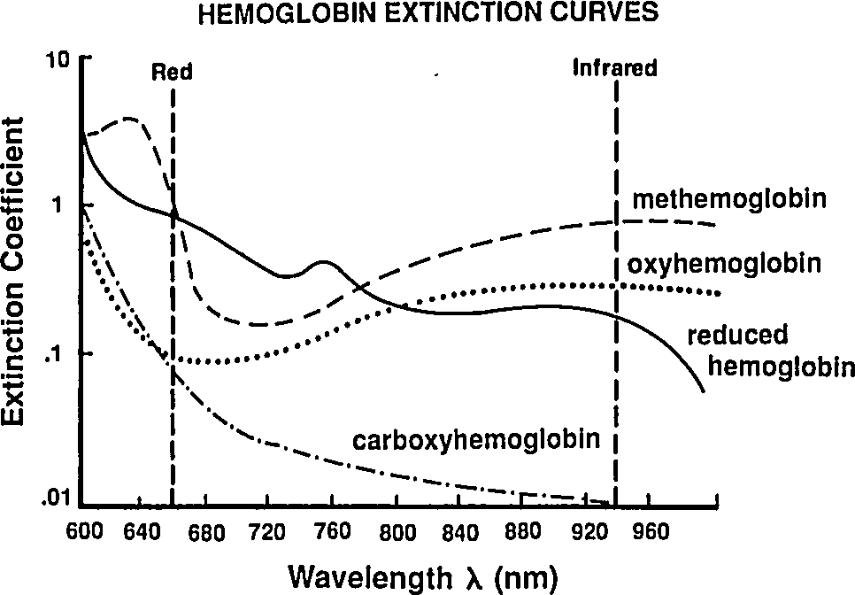
So far we've been labeling and defining attributes of the blood. The point of this excercise is to understand how a pulse oximeter measures them. People have known for a while that different hemoglobin complexes (HbO₂, HHb, MHb, HbCO, …) have differnt absorbtion spectra, and they have been using this difference since the 1930's to make pulse-oximeters based on two-color transmittance measurements (see Tremper 1989).

Absorbance spectra for assorted hemoglobin species (Tremper 1989)

By passing different wavelengths of light through perfused tissue, we can measure the relative quantities of the different Hb species. The basis for this analysis comes from the Beer-Lambert law.

(8)

I = I_{0} e^{- c ϵ L},

where $I_{0}$ is the incident intensity (entering the tissue), $I$ is the tranmitted intensity (leaving the tissue), $c$ is the tissue density (concentration), $ϵ$ is the extinction coefficient (molar absorbtivity), and $L$ is the tissue thickness. Rephrasing the math as English, this means that the intensity drops off exponentially as you pass through the tissue, and more tissue (higher $c$ or $L$ ) or more opaque tissue (higher $ϵ$ ) mean you'll get less light out the far side. This is a very simple law, and the price of the simplicity is that it brushes all sorts of things under the rug. Still, it will help give us a basic idea of what is going on in a pulse-oximeter.

Rather than treat the the tissue as a single substance, lets use the Beer-Labmert law on a mixture of substances with concentrations $c_{1}$ , $c_{2}$ , … and extinction coefficients $ϵ_{1}$ , $ϵ_{2}$ , ….

(9)

I = I_{0} e^{- (c_{1} ϵ_{1} + c_{2} ϵ_{2} + \dots) L} .

We also notice that the intensities and extinction coefficients may all depend on the wavelength of light $λ$ , so we should really write

(10)

I_{λ} = I_{0 λ} e^{- (c_{1} ϵ_{1 λ} + c_{2} ϵ_{2 λ} + \dots) L} .

Once isolated, a simple spectroscopy experiment can measure the extinction coefficient $ϵ_{i λ}$ of a given species across a range of $λ$ , and this has been done for all of our common Hb flavors. We need to play with the last equation to find a way to extract the unknown concentrations, which we can then use to calculate the ${Sf}_{O₂}$ and $S_{O₂}$ which we can use in turn to calculate $[O₂]$ .

Note that by increasing the number of LEDs (adding new $λ$ ) we increase the number of constraints on the unknown $c_{i}$ . A traditional pulse-oximeter uses two LEDs, at 660 nm and 940 nm, to measure ${Sf}_{O₂}$ (related to [HbO₂] and [HHb]). More recent designs called pulse CO-oximeters use more wavelengths to allow measurement of quanties related to additional species (approaching the end goal of measuring $S_{O₂}$ ).

Let us deal with the fact that there is a lot of stuff absorbing light that is not arterial blood (e.g. venous blood, other tissue, bone, etc). The good thing about this stuff is that it's just sitting there or moving through in a smooth fasion. Arterial blood is the only thing that's pulsing. Here's another figure from Tremper:

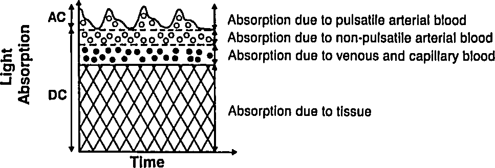AC and DC transmission components (Tremper)

During a pulse, the pressure in the finger increases and non-arterial tissue is compressed, changing $L$ and $c_{i}$ from their trough values to peak values $L'$ and $c_{i}'$ . Since the finger is big, the fractional change in width $d L / L = (L' - L) / L$ is very small. Assuming the change in concentration is even smaller (since most liquids are fairly incompressible), we have

(11)

\begin{aligned} \frac{d I_{λ}}{d L} & = \frac{d}{d L} (I_{0 λ} e^{- (c_{1} ϵ_{1 λ} + c_{2} ϵ_{2 λ} + \dots) L}) = \frac{d}{d L} (I_{0 λ} e^{- X L}) = - X I_{0 λ} e^{- X L} = - {XI}_{λ} \\ \frac{d I_{λ}}{I_{λ}} & = - X d L, \end{aligned}

where $X = c_{1} ϵ_{1 λ} + c_{2} ϵ_{2 labmda} + \dots$ is just a placeholder to reduce clutter. $d I_{λ}$ is the AC amplitude (height of wiggle top of the detected light intensity due to pulsatile arterial blood), while $I_{λ}$ is the DC ampltude (height of the static base of the detected light intensity due to everything else). This is actually a fairly sneaky step, because if we can also use it to drop the DC compents. Because we've assumed fixed concentrations (incompressible fluids), and there is no more DC material coming in during a pulse (by definition), the effective $L$ for the DC components does not change. Separating the DC and AC components and running through the derivative again, we have

(12)

\begin{aligned} \frac{d I_{λ}}{d L} & = \frac{d}{d L} (I_{0 λ} e^{- (c_{DC 1} ϵ_{DC 1 λ} + c_{DC 2} ϵ_{DC 2 λ} + \dots) L_{DC} - (c_{AC 1} ϵ_{AC 1 λ} + c_{AC 2} ϵ_{AC 2 λ} + \dots) L_{AC}}) \\ = I_{0 λ} e^{- (c_{DC 1} ϵ_{DC 1 λ} + c_{DC 2} ϵ_{DC 2 λ} + \dots) L_{DC}} \frac{d}{d L} (e^{- (c_{AC 1} ϵ_{AC 1 λ} + c_{AC 2} ϵ_{AC 2 λ} + \dots) L_{AC}}) \\ = I_{0 λ} Y \frac{d}{d L} (e^{- Z L_{AC}}) = - Z I_{0 λ} Y e^{- Z L_{AC}} = - Z I_{λ} \\ \frac{d I_{λ}}{I_{λ}} & = - Z d L, \end{aligned}

where $Y = e^{- (c_{DC 1} ϵ_{DC 1 λ} + c_{DC 2} ϵ_{DC 2 λ} + \dots) L_{DC}}$ and $Z = c_{AC 1} ϵ_{AC 1 λ} + c_{AC 2} ϵ_{AC 2 λ} + \dots)$ are just placeholders to reduce clutter. Note that the last equation looks just like the previous one with the translation $X \to Z$ . This means that if we stick to using the AC-DC intensity ratio ( $\frac{d Il}{Il}$ ) we can forget about the DC contribution completely.

If the changing- $L$ -but-static- $L_{DC}$ thing bothers you, you can imagine insteadthat $L_{DC}$ grows with $L$ , but $c_{DC i}$ shrinks proportially (to conserve mass). With this proportionate stretching, there is still no change in absorbtion for that component so $\frac{d}{d L} \exp (- c_{DC i} ϵ_{DC i λ} L) = 0$ and we can still pull the DC terms out of the integral as we just did.

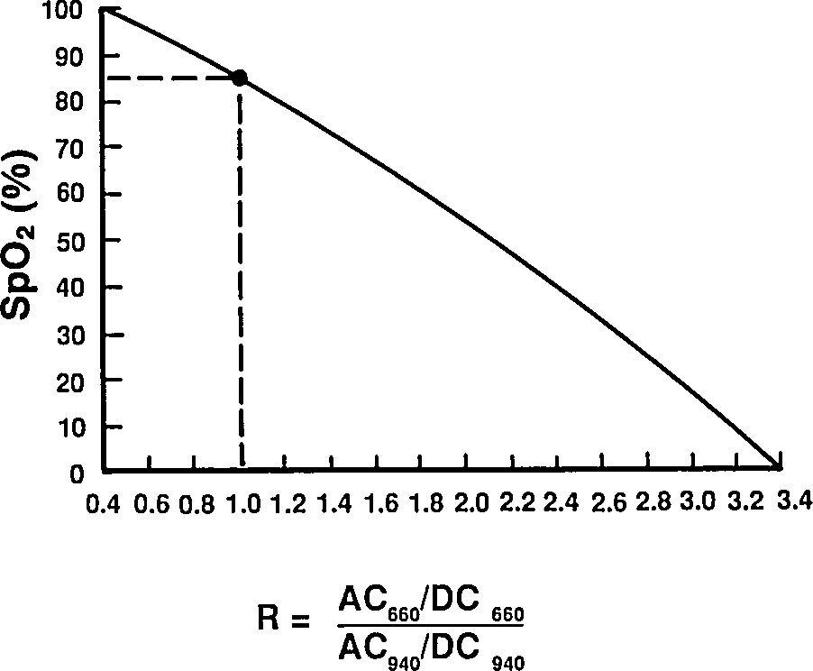
Taking a ratio of these amplitudes at two different wavelengths, we get optical density ratio (R)

(13)

R = \frac{\frac{{AC}_{660}}{{DC}_{660}}}{\frac{{AC}_{940}}{{DC}_{940}}} = \frac{\frac{d I_{660}}{I_{660}}}{\frac{d I_{940}}{I_{940}}} = \frac{- Z_{660} d L}{- Z_{940} d L} = \frac{Z_{660}}{Z_{940}},

because $d L$ (the amount of finger expansion during a pulse) obviously doesn't depend on the color light you are using. Plugging back in for $Z$ ,

(14)

R = \frac{c_{AC 1} ϵ_{AC 1,660} + c_{AC 2} ϵ_{AC 2,660} + \dots}{c_{AC 1} ϵ_{AC 1,940} + c_{AC 2} ϵ_{AC 2,940} + \dots}

Assuming, for now, that there are only two species of Hb—HbO₂ and HHb—we can solve for $c_{AC 1} / c_{AC 2}$ .

(15)

\begin{aligned} R & = \frac{c_{AC 1} ϵ_{AC 1,660} + c_{AC 2} ϵ_{AC 2,660}}{c_{AC 1} ϵ_{AC 1,940} + c_{AC 2} ϵ_{AC 2,940}} \\ R (c_{AC 1} ϵ_{AC 1,940} + c_{AC 2} ϵ_{AC 2,940}) & = c_{AC 1} ϵ_{AC 1,660} + c_{AC 2} ϵ_{AC 2,660} \\ c_{AC 1} (R ϵ_{AC 1,940} - ϵ_{AC 1,660}) & = c_{AC 2} (ϵ_{AC 2,660} - R ϵ_{AC 2,940}) \\ \frac{c_{AC 1}}{c_{AC 2}} & = \frac{ϵ_{AC 2,660} - R ϵ_{AC 2,940}}{R ϵ_{AC 1,940} - ϵ_{AC 1,660}} . \end{aligned}

So now we know [HbO₂]/[HHb] in terms of the measured quantity $R$ and the empirical values $ϵ$ .

Plugging in to our equation for ${Sf}_{O₂}$ to find the functional saturation:

(16)

\begin{aligned} {Sf}_{O₂} & = \frac{[HbO₂]}{[HbO₂] + [HHb]} = \frac{1}{1 + \frac{[HHb]}{[HbO₂]}} = \frac{1}{1 + \frac{c_{AC 2}}{c_{AC 1}}} = \frac{1}{1 + \frac{R ϵ_{AC 1,940} - ϵ_{AC 1,660}}{ϵ_{AC 2,660} - R ϵ_{AC 2,940}}} . \end{aligned}

As a check, we can rephrase this as

(17)

\begin{aligned} {Sf}_{O₂} & = \frac{1}{1 + \frac{R ϵ_{AC 1,940} - ϵ_{AC 1,660}}{ϵ_{AC 2,660} - R ϵ_{AC 2,940}}} = \frac{ϵ_{AC 2,660} - R ϵ_{AC 2,940}}{ϵ_{AC 2,660} - R ϵ_{AC 2,940} + R ϵ_{AC 1,940} - ϵ_{AC 1,660}} \\ = \frac{ϵ_{AC 2,660} - R ϵ_{AC 2,940}}{ϵ_{AC 2,660} - ϵ_{AC 1,660} + (ϵ_{AC 1,940} - ϵ_{AC 2,940}) R} = \frac{- ϵ_{AC 2,660} + ϵ_{AC 2,940} R}{ϵ_{AC 1,660} - ϵ_{AC 2,660} + (ϵ_{AC 2,940} - ϵ_{AC 1,940}) R}, \end{aligned}

which matches Mendelson 1989, Eq. 8 with the translations:

${Sf}_{O₂} \to Sp O₂$ ,
$R \to R / IR$ ,
$ϵ_{AC 2,660} \to ϵ_{R} (Hb)$ ,
$ϵ_{AC 2,940} \to ϵ_{IR} (Hb)$ ,
$ϵ_{AC 1,660} \to ϵ_{R} (HbO₂)$ , and
$ϵ_{AC 1,940} \to ϵ_{IR} (HbO₂)$ .

And that is the first-order explaination of how a pulse-oximeter measures the functional saturation!

Reading extinction coefficients off the absorbtion figure, I get

(18)

\begin{aligned} ϵ_{HbO₂, 660} & = ϵ_{AC 1,660} = 0.10 \\ ϵ_{HHb, 660} & = ϵ_{AC 2,660} = 0.83 \\ ϵ_{HbO₂, 940} & = ϵ_{AC 1,940} = 0.29 \\ ϵ_{HHb, 940} & = ϵ_{AC 2,940} = 0.17 \end{aligned}

which are comfortingly close to those given by Mendelson in Table 1. The corresponding ${Sf}_{O₂} (R)$ plot (from Tremper) is:

Experimental SpO₂ vs. R (Tremper)

Theoretical SfO₂ vs. R.

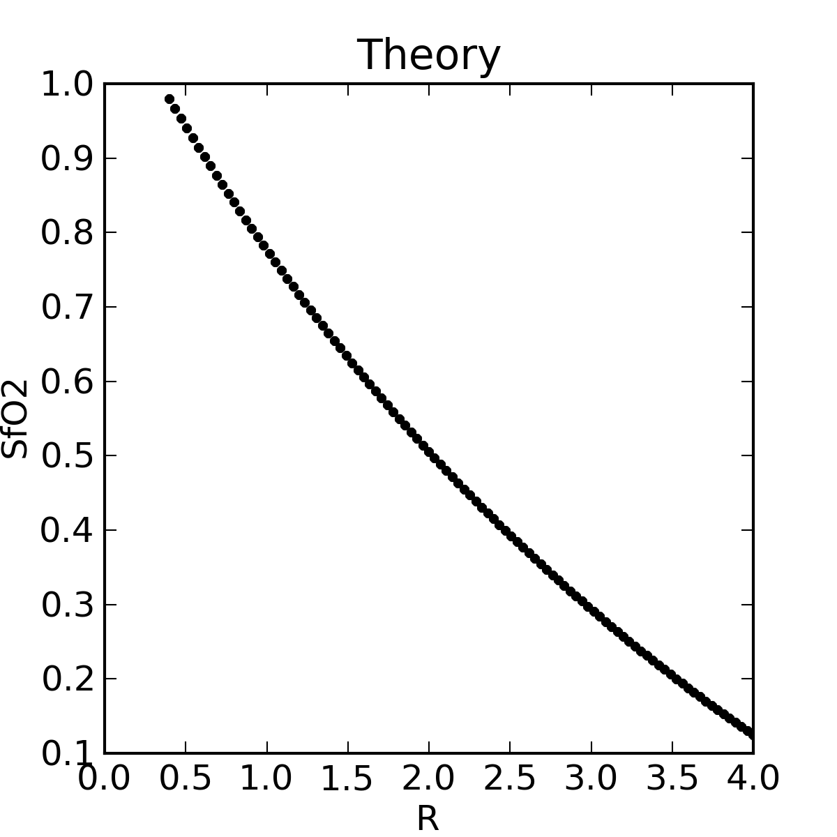The theoretical plot was calculated using SfO2vR-theory.py and our ${Sf}_{O₂}$ equation. This is why it’s a good idea to use an empirical calibration curve! The concave theoretical curve is supported by Mendelson's figure 4.

Nomenclature

O₂: Molecular oxygen
[ $x$ ]: Concentration of $x$ in the blood
BTP: Body temperature and pressure
STP: Standard temperature and pressure
$P_{O₂}$: O₂ partial pressure
$P i_{O₂}$: O₂ partial pressure at location $i$
$S_{O₂}$: Fractional O₂ saturation
$S i_{O₂}$: O₂ fractional saturation at location $i$
${Sf}_{O₂}$: Functional O₂ saturation
Hg: Mercury
Hb: Hemoglobin monomer
HbO₂: Hemoglobin monomers complexed with O₂
HHb: Reduced hemoglobin (not complexed with O₂)
dysHb: Dys-hemoglobin (cannot complex with O₂)
MHb: Methemoglobin
HbCO: Carboxyhemoglobin
$I_{0 λ}$: Intensity of incident light at wavelength $λ$
$I_{λ}$: Intensity of transmitted light at wavelength $λ$
$c_{i}$: Concentration of light-absorbing species $i$
$c_{DC i}$: Concentration of the $i$ th DC species at wavelength $λ$
$c_{AC i}$: Concentration of the $i$ th AC species at wavelength $λ$
$ϵ_{i λ}$: Extinction coefficient of species $i$ at wavelength $λ$
$ϵ_{DC i λ}$: Extinction coefficient of the $i$ th DC species wavelength $λ$
$ϵ_{DC i λ}$: Extinction coefficient of the $i$ th DC species wavelength $λ$
$L$: Length of tissue through which light must pass
$L_{DC}$: Diastolic finger width
$R$: Optical density ratio
LED: Light emitting diode

Over the last few days I've been trying to teach myself enough genetics to reconstruct Carrion-Vazquez's poly-I27 synthesis procedure. I'm not quite there yet, but I feel like I've made enough progress that it's worth posting my notes somewhere public in case they are useful to others.

Overview

We buy our poly-I27 from AthenaES, who market it as I27O™. Perusing their technical brief, makes it clear that I2O7™ corresponds to Carrion-Vazquez's I27^RS₈. In Carrion-Vazquez' original paper they describe the synthesis of both I27^RS₈ and a variant I27^GLG₁₂. Their I27^RS₈ procedure is:

Human cardiac muscle used to generate a cDNA library (Rief 1997)
cDNA library amplified with PCR
- 5' primer contained a BamHI restriction site that permitted in-frame cloning of the monomer into the expression vector pQE30.
- The 3' primer contained a BglII restriction site, two Cys codons located 3' to the BglII site and in-frame with the I27 domain, and two in-frame stop codons.
The PCR product was cloned into pUC19 linearized with BamHI and SmaI.
The 8-domain synthetic gene was constructed by iterative cloning of monomer into monomer, dimer into dimer, and tetramer into tetramer.
The final construct contained eight direct repeats of the I27 domain, an amino-terminal His tag for purification, and two carboxyl-terminal Cys codons used for covalent attachment to the gold-covered coverslips.

They also give the full-length sequence of I27^RS₈:

Met-Arg-Gly-Ser-(His)₆-Gly-Ser-(I27-Arg-Ser)₇-I27-...-Cys-Cys

They point out the Arg-Ser (RS) amino acid sequence is the BglII/BamHI hybrid site, which makes sense.

Back on the Athena site, they have a page describing their procedure (they reference the Carrion-Vazquez paper). They claim to use the restriction enzyme KpnI in addition to BamHI, BglII, and SmaI.

Carrion-Vazquez points to the following references:

Kempe et al. 1985 (CV16), the source of the multi-step cloning technique.
Rief et al. (CV10), for I27 subcloning.

Rief

In their note 11, Rief et al. explain their synthesis procedure:

λ cDNA library
Titin fragments of interest were amplified by PCR
cloned into pET 9d
NH₂-terminal domain boundaries were as in Politou 1996.
The clones were fused with an NH₂-terminal His₆ tag and a COOH-terminal Cys₂ tag for immobilization on solid surfaces.

which doesn't help me very much.

Kemp

The Kempe article is more informative, focusing entirely on the synthesis procedure (albiet for a different gene). Their figure 2 outlines the general approach, and used the following restriction enzymes: PstI, BamHI, PstI, and BglII. I'll walk through their procedure in detail below.

Genetic code

Wikipedia has a good page on the genetic code for converting between DNA/mRNA codons and amino acids. I've written up a little Python script, mRNAcode.py, to automate the conversion of various sequences, which helped me while I was writing this post. I'm sure there are tons of similar programs out there, so don't feel pressured to use mine ;).

Restriction enzymes

We'll use the following restriction enzymes:

BamHI

5' G|GATC C 3'
3' C CTAG|G 5'

BglI (N is any nucleotide)

5' GCCN NNN|NGGC 3'
3' CGGN|NNN NCCG 5'

BglII

5' A|GATC T 3'
3' T CTAG|A 5'

HindIII

5' A|AGCT T 3'
3' T TCGA|A 5'

KpnI

5' G GTAC|C 3'
3' C|CATG G 5'

PstI

5' C TGCA|G 3'
3' G|ACGT C 5'

SmaI

5' CCC|GGG 3'
3' GGG|CCC 5'

Details

Here's my attempt to reconstruct the details of the polymer-cloning reactions, where they splice several copies of I27 into the expression plasmid.

Kempe procedure

Inserted their poly-SP into pHK414 (I haven't been able to find any online sources for pHK414. Kempe cites R.J. Watson et al. Expression of Herpes simplex virus type 1 and type 2 glyco-protein D genes using the Escherichia coli lac promoter. Y. Becker (Ed.), Recombinant DNA Research and Viruses. Nijhoff, The Hague, 1985, pp. 327-352.)

Synthetic SP

     HindIII.                                                ,BamHI_.
     |      |  Met Arg Pro Lys Pro Gln Gln Phe Phe Gly Leu Met      |
 5’ GA AGC TTC ATG CGT CCG AAG CCG CAG CAG TTC TTC GGT CTC ATG GAT CCG
    CT TCG AAG TAC GCA GGC TTC GGC GTC GTC AAG AAG CCA GAG TAC CTA GGC 5’

pHK414

          _______Linker_sequence______
         /                            \
               HindIII    BamHI
,PstI.   BglII.|    |,SmaI.    |
CTGCAG...AGATCTAAGCTTCCCGGGGATCCAAGATCC
GACGTC...TCTAGATTCGAAGGGCCCCTAGGTTCTAGG
.                                     .
.......................................

Synthesizing pSP4-1

pHK414 + HindIII + BamHI

They cut a hole in the plasmid…

               HindIII    BamHI.
(PstI)   BglII,|               |
CTGCAG...AGATCTA           GATCCAAGATCC
GACGTC...TCTAGATTCGA           GTTCTAGG
.                                     .
.......................................

SP + HindIII + BamHI

… and cut matching snips off their SP gene.

HindIII.                                                ,BamHI_.
|      |  Met Arg Pro Lys Pro Gln Gln Phe Phe Gly Leu Met      |
  AGC TTC ATG CGT CCG AAG CCG CAG CAG TTC TTC GGT CTC ATG
       AG TAC GCA GGC TTC GGC GTC GTC AAG AAG CCA GAG TAC CTA G

pSP4-1

Mixing the snips together gives the plasmid with a single SP.

               HindIII                                   BamHI.
,PstI.   BglII.|    | MetArgProLysProGlnGlnPhePheGlyLeuMet    |
CTGCAG...AGATCTAAGCTTCATGCGTCCGAAGCCGCAGCAGTTCTTCGGTCTCATGGATCCAAGATCC
GACGTC...TCTAGATTCGAAGTACGCAGGCTTCGGCGTCGTCAAGAAGCCAGAGTACCTAGGTTCTAGG
.                                                                    .
......................................................................

Using -SP- to abbreviate the HindIII→Met→Met portion (less the terminal G, which is part of the BamHI match sequence).

,PstI.   BglII.    BamHI.
CTGCAG...AGATCT-SP-GGATCC
GACGTC...TCTAGA-SP-CCTAGG
.                       .
.........................

Synthesizing pSP4-2

The single-SP plasmid, pSP4-1, is split in two parallel reactions.

PstI + BamHI

    G...AGATCT-SP-G
ACGTC...TCTAGA-SP-CCTAG

PstI + BglII

CTGCA     GATCT-SP-GGATCC
G             A-SP-CCTAGG
.                       .
.........................

pSP4-2

Then the SP-containing fragments (shown above) are isolated and mixed together to form pSP4-2.

,PstI.   BglII.    other.    BamHI.
CTGCAG...AGATCT-SP-GGATCT-SP-GGATCC
GACGTC...TCTAGA-SP-CCTAGA-SP-CCTAGG
.                                 .
...................................

where the "other" sequence is the result of the BamHI/BglII splice. Expanding the -SP- abbreviation around the SP joint:

....SP,other_.HindIII.  SP.....
Leu Met Asp Leu Ser Phe Met Arg
CTC ATG GAT CTA AGC TTC ATG CGT
AGA CGT TCG AGC CTA GGA CGT ATG

So the resulting poly-SP will have Asp-Leu-Ser-Phe linking amino acids.

By repeating the PstI + BamHI / PstI + BglII split-and-join, you can synthesize plasmids with any number of SP repeats.

I27^RS₈ procedure

Like Kempe, Carrion-Vazquez et al. flank the I27 gene with BglII and BamHI, but they reverse the order. Here's the output of their PCR:

BamHI-I27-BglII-Cys-Cys-STOP-STOP

From the PDB entry for I27 (1TIT), the amino acid sequence is:

,leader_.
MHHHHHHSSLIEVEKPLYGVEVFVGETAHFEIELSEPDVHGQWKLKGQPLTASPDCEIIEDGKKHILI
LHNCQLGMTGEVSFQAANAKSAANLKVKEL

To translate this into cDNA, I've scanned thorough the sequence of NM_003319.4, and found a close match from nucleotides 15991 through 16248.

15982 CTAATAAAAG TGGAAAAGCC TCTGTACGGA GTAGAGGTGT TTGTTGGTGA
16032 AACAGCCCAC TTTGAAATTG AACTTTCTGA ACCTGATGTT CACGGCCAGT
16082 GGAAGCTGAA AGGACAGCCT TTGACAGCTT CCCCTGACTG TGAAATCATT
16132 GAGGATGGAA AGAAGCATAT TCTGATCCTT CATAACTGTC AGCTGGGTAT
16182 GACAGGAGAG GTTTCCTTCC AGGCTGCTAA TGCCAAATCT GCAGCCAATC
16232 TGAAAGTGAA AGAATTG

This cDNA match generates an amino acid starting with LIKVEK instead of the expected LIEVEK, but the LIKVEK version matches amino acids 12677-12765 in Q8WZ42 (canonical titin), and there is a natural variant listed for 12679 K→E.

Interestingly, this sequence contains a PstI site at nucleotides 16220 through 16225. None of our other restriction enzymes have sites in the I27 sequence.

Carrion-Vazquez et al. list two vectors in their procedure, but I'm not sure about their respective roles.

pQE30

pQE30 (sequence) is listed as the "expression vector", but I'm not sure why they would need a non-expression vector, as they don't reference cross-vector subcloning after inserting their I27 monomer into the plasmid.

From the Qiagen site, the section around the linker nucleotides 115 through 203 is:

    ,RGS-His epitope__________________. ,BamHI.
Met Arg Gly Ser His His His His His His Gly Ser Ala Cys Glu Leu
ATG AGA GGA TCG CAT CAC CAT CAC CAT CAC GGA TCC GCA TGC GAG CTC
CGT CTC TTC GAT ACG ACA ACG ACA ACG ACA TTC GAA TAC GTA TCT AGA

      ,SmaI__.
,KpnI_.                         HindIII
Gly Thr Pro Gly Arg Pro Ala Ala Lys Leu Asn STOP
GGT ACC CCG GGT CGA CCT GCA GCC AAG CTT AAT TAG CTG AG
TTG CAA AAT TTG ATC AAG TAC TAA CCT AGG CCG GCT AGT CT

However, there is no BglII site in this linker. In fact, there is no BglII site in the entire pQE30 plasmid, so they'd need to use a third restiction enzyme to insert their I27 (which does contain a trailing BglII).

pUC19

From BCCM/LMBP and GenBank, the section around the linker nucleotides 233 through 289 is:

                                                 ,SmaI_.
HindIII.        ,PstI__.                ,BamHI_.    ,KpnI__.
           Met                     STOP
AA GCT TGC ATG CCT GCA GGT CGA CTC TAG AGG ATC CCC GGG TAC CGA

GCT CGA ATT C

However, there is no BglII the entire pUC19 plasmid either, so they'd need to use a third restiction enzyme to insert their I27.

Questions

Why do Carrion-Vazquez et al. list two different plasmids?
What is the 3'-side restiction enzyme that Carrion-Vazquez et al. use to insert their I27 into their plasmid?
What is the remote restriction enzyme that Carrion-Vazquez et al. use to break their opened plasmids (Kempe PstI equivalent).
The BamHI and SmaI sites in pUC19 overlap, so it is unclear how you could use both to "linearize" pUC19. It would seem that either one would open the plasmid on its own, although I'm not sure you could "heal" the blunt-ended SmaI cut.
Since the Arg-Ser joint is formed by a BglII/BamHI overlap, why are there no BglII-coded amino acids after the last I27 in the I27^RS₈ sequence? If there is, why do Carrion-Vazquez et al. not acknowledge it when they write [3]:

The full-length construct, I27^RS₈, results in the following amino acid additions: (i) the amino-terminal sequence is Met-Arg-Gly-Ser-(His)6-Gly-Ser-I27 codons; (ii) the junction between the domains (BamHI-BglII hybrid site) is Arg-Ser; and (iii) the protein terminates in Cys-Cys.

Since they don't acknowledge an I27-Arg-Ser-Cys-Cys ending, might there be more amino acids in the C terminal addition?

Working backward

Since I'm stuck trying to get I27 into either plasmid, let's try and work backward from

Met-Arg-Gly-Ser-(His)₆-Gly-Ser-(I27-Arg-Ser)₇-I27-...-Cys-Cys

BglII/BamHI joint

The BglII/BamHI overlap would produce the expected Arg-Ser joint.

BglII   BamHI
A     + GATCC = AGATCC = Arg-Ser
TCTAG       G   TCTAGG

Final plasmid (pI27-8)

The beginning of this sequence looks like the start of pQE30's linker, so we'll assume the final plasmid was:

remote ...    ,RGS-His epitope__________________. ,BamHI. I27...
       ... Met Arg Gly Ser His His His His His His Gly Ser Leu Ile ...
???    ... ATG AGA GGA TCG CAT CAC CAT CAC CAT CAC GGA TCC CTA ATA ...
???    ... CGT CTC TTC GAT ACG ACA ACG ACA ACG ACA TTC GAA GAT TAT ...

........I27 joint_. I27 ... final I27 ,BglII.                 continuation of pQE30?
... Glu Leu         Leu ...       Leu Arg Ser Cys Cys STOPSTOP...
... GAA TTG AGA TCC CTA ...       TTG AGA TCT TGC TGC TAG TAG ...
... CTT AAC TCT AGG GAT ...       GAT CTC GAG GTA GTA GCT GCT ...

Penultimate plasmid (pI27-4)

remote ...    ,RGS-His epitope__________________. ,BamHI. I27...
           Met Arg Gly Ser His His His His His His Gly Ser Leu Ile ...
???    ... ATG AGA GGA TCG CAT CAC CAT CAC CAT CAC GGA TCC CTA ATA ...
???    ... CGT CTC TTC GAT ACG ACA ACG ACA ACG ACA TTC GAA GAT TAT ...

    ... I27 joint_. I27 ... fourth I27 ,BglII.                 continuation of pQE30?
... Glu Leu         Leu ...        Leu Arg Ser Cys Cys STOPSTOP...
... GAA TTG AGA TCC CTA ...        TTG AGA TCT TGC TGC TAG TAG ...
... CTT AAC TCT AGG GAT ...        GAT CTC GAG GTA GTA GCT GCT ...

pI27-4 + BamHI + remote

remote                                             ,BamHI. I27...
                                                           Leu Ile ...
?                                                   GA TCC CTA ATA ...
??                                                       A GAT TAT ...

....... I27 joint_. I27 ... fourth I27 ,BglII.                 continuation of pQE30?
... Glu Leu         Leu ...        Leu Arg Ser Cys Cys STOPSTOP...
... GAA TTG AGA TCC CTA ...        TTG AGA TCT TGC TGC TAG TAG ...
... CTT AAC TCT AGG GAT ...        GAT CTC GAG GTA GTA GCT GCT ...

pI27-4 + BglII + remote

remote ...    ,RGS-His epitope__________________. ,BamHI. I27...
           Met Arg Gly Ser His His His His His His Gly Ser Leu Ile ...
 ??    ... ATG AGA GGA TCG CAT CAC CAT CAC CAT CAC GGA TCC CTA ATA ...
  ?    ... CGT CTC TTC GAT ACG ACA ACG ACA ACG ACA TTC GAA GAT TAT ...

....... I27 joint_. I27 ... fourth I27 ,BglII.
... Glu Leu         Leu ...        Leu
... GAA TTG AGA TCC CTA ...        TTG A
... CTT AAC TCT AGG GAT ...        GAT CTC GA

pI27-8

remote ...    ,RGS-His epitope__________________. ,BamHI. I27...
           Met Arg Gly Ser His His His His His His Gly Ser Leu Ile ...
???    ... ATG AGA GGA TCG CAT CAC CAT CAC CAT CAC GGA TCC CTA ATA ...
???    ... CGT CTC TTC GAT ACG ACA ACG ACA ACG ACA TTC GAA GAT TAT ...

....... I27 joint_. I27 ... fourth I27 ,other. I27...
... Glu Leu         Leu ...        Leu Gly Ser Leu Ile ...
... GAA TTG AGA TCC CTA ...        TTG AGA TCC CTA ATA ...
... CTT AAC TCT AGG GAT ...        GAT CTC GAA GAT TAT ...

....... I27 joint_. I27 ... fourth I27 ,BglII.                 continuation of pQE30?
... Glu Leu         Leu ...        Leu Arg Ser Cys Cys STOPSTOP...
... GAA TTG AGA TCC CTA ...        TTG AGA TCT TGC TGC TAG TAG ...
... CTT AAC TCT AGG GAT ...        GAT CTC GAG GTA GTA GCT GCT ...

Continuing to the first plasmid, pI27-1 must have been

remote ...    ,RGS-His epitope__________________. ,BamHI. I27...
       ... Met Arg Gly Ser His His His His His His Gly Ser Leu Ile ...
???    ... ATG AGA GGA TCG CAT CAC CAT CAC CAT CAC GGA TCC CTA ATA ...
???    ... CGT CTC TTC GAT ACG ACA ACG ACA ACG ACA TTC GAA GAT TAT ...

........I27 ,BglII.                 continuation of pQE30?
... Glu Leu Arg Ser Cys Cys STOPSTOP...
... GAA TTG AGA TCT TGC TGC TAG TAG ...
... CTT AAC CTC GAG GTA GTA GCT GCT ...

Potential pQE30 insertion points

Kpn1 (present after BamHI in both plasmids)

Potential remote restriction enzymes

BglI (pQE30 nucleotides 2583-2593 (GCCGGAAGGGC), Amp-resistance 3256-2396; pUC19 has two BglI sites (bad idea))

Available in a git repository.
Repository: pypid
Browsable repository: pypid
Author: W. Trevor King

I've just finished rewriting my PID temperature control package in pure-Python, and it's now clean enough to go up on PyPI. Features:

Backend-agnostic architecture. I've written a first-order process with dead time (FOPDT) test backend and a pymodbus-based backend for our Melcor MTCA controller, but it should be easy to plug in your own custom backend.
The general PID controller will automatically tune your backend using any of a variety of tuning rules.

The README is posted on the PyPI page.

There are a number of open source packages dealing with aspects of single-molecule force spectroscopy. Here's a list of everything I've heard about to date (for more details on calibcant, Hooke, and sawsim, see my thesis).

Package	License	Purpose
calibcant	GPL v3+	Cantilever thermal calibration
fs_kit	GPL v2+	Force spectra analysis pattern recognition
Hooke	LGPL v3+	Force spectra analysis and unfolding force extraction
sawsim	GPL v3+	Monte Carlo unfolding/refolding simulation and fitting
refolding	Apache v2.0	Double-pulse experiment control and analysis

calibcant

Calibcant is my Python module for AFM cantilever calibration via the thermal tune method. It's based on Comedi, so it needs work if you want to use it on a non-Linux system. If you're running a Linux kernel, it should be pretty easy to get it running on your system. Email me if there's any way I can help set it up for your lab.

fs_kit

fs_kit is a package for force spectra analysis pattern recognition. It was developed by Michael Kuhn and Maurice Hubain at Daniel Müller's lab when they were at TU Dresden (paper). It has an Igor interface, but the bulk of the project is in C++ with a wxWidgets interface. fs_kit is versioned in CVS at bioinformatics.org, and you can check out their code with:

$ cvs -d:pserver:anonymous@bioinformatics.org:/cvsroot checkout fskit

The last commit was on 2005/05/16, so it's a bit crusty. I patched things up back in 2008 so it would compile again,

0001-Added-math.h-include-to-fs align histogram2d.h.patch
Posted Sat 23 Apr 2011 11:57:47 AM PDT

0002-changed-abs-double-to-fabs-double-in-fs fit spectr.patch
Posted Sat 23 Apr 2011 11:57:47 AM PDT

0003-Updated-wxWindows-code-to-compile-on-wx-2.8.patch
Posted Sat 23 Apr 2011 11:57:47 AM PDT

0004-Added-wxglade-entry-to-Makefile-for-regenerating-aut.patch
Posted Sat 23 Apr 2011 11:57:47 AM PDT

but when I emailed Michael with the patches I got this:

On Thu, Oct 23, 2008 at 11:21:42PM +0200, Michael Kuhn wrote:
> Hi Trevor,
>
> I'm glad you could fix fs-kit, the project is otherwise pretty dead,
> as was the link. I found an old file which should be the tutorial,
> hopefully in the latest version. The PDF is probably lost.
>
> bw, Michael

So, it's a bit of a fixer-upper, but it was the first open source package in this field that I know of. I've put up a PDF version of the tutorial Michael sent me in case you're interested.

Hooke

Hooke is a force spectroscopy data analysis package written in Python. It was initially developed by Massimo Sandal, Fabrizio Benedetti, Marco Brucale, Alberto Gomez-Casado while at Bruno Samorì's lab at U Bologna (paper; surprisingly, there are commits by all of the authors except Samorì himself). Hooke provides the interface between your raw data and theory. It has a drivers for reading most force spectroscopy file formats, and a large number of commands for manipulating and analyzing the data.

I liked Hooke so much I threw out my already-written package that had been performing a similar role and proceeded to work over Hooke to merge together the diverging command-line and GUI forks. Unfortunately, my fork has not yet been merged back in as the main branch, but I'm optimistic that it will eventually. The homepage for my branch is here.

sawsim

While programs like Hooke can extract unfolding forces from velocity-clamp experiments, the unfolding force histograms are generally compared to simulated data to estimate the underlying kinetic parameters. Sawsim is my package for performing such simulations and fitting them to the experimental histograms (paper). The single-pull simulator is written in C, and there is a nice Python wrapper that manages the thousands of simulated pulls needed to explore the possible model parameter space. The whole package ends up being pretty fast, flexible, and convenient.

refolding

Refolding is a suite for performing and analyzing double-pulse refolding experiments. It was initially developed by Daniel Aioanei, also at the Samorí lab in Bologna (these guys are great!). The experiment-driver is mostly written in Java with the analysis code in Python. The driver is curious; it uses the NanoScope scripting interface to drive the experiment through the NanoScope software by impersonating a mouse-wielding user (like Selenium does for web browsers). See the RobotNanoDriver.java code for details. There is also support for automatic velocity clamp analysis.

The official paper for the project is by Aioanei. The earlier paper by Materassi may be related, but Aioanei doesn't cite it in his paper, and Materassi doesn't give a URL for his code.

Hardware

Nice software doesn't do you much good if you don't have the hardware to control. There are a number of quasi-open hardware solutions for building your own AFM (and other types of scanning probe microscopes). There's a good list on opencircuits. Interesting projects include:

Glenn Durden's STM (1992–1998)
Jim Rice's Homebrew STM (1995)
The Peddie School's STM Project (1997–2002)
Jürgen Müller's home-built STMs (1999–2006)
John D. Alexander's STM Project (2000–2003)
The Münster Interface Physics Group's SXM Project (free except for commercial use, 2000–2005).
Joseph Gatt's Amateur STM (2003)
Maxim Shusteff's AFM for the instructional laboratory (2006)
Dominik, Ivan, and Sandro's STM-DIY project (2009)

Other software

The Gnome X Scanning Miscroscopy (GXSM) project provides GPL software to perform standard SPM imaging. The list of supported hardware is currently limited to the SignalRanger series by SoftdB, via GXSM-specific kernel modules like sranger-mk23-dkms. There is an obsolete Comedi driver for GXSM that Percy Zahl wrote back in 1999, but it has been deprecated since at least 2007.

Force spectroscopy is the process of extracting information about the unfolding (or unbinding) characteristics of a protein (or ligand-receptor pair) by measuring force vs. extension curves while gradually ripping the protein (or pair) apart. Consider this cartoon representation of the procedure

The AFM tip is pulling a protein chain away from the substrate, causing one of the protein domains to uncoil.

The procedure yields 'force curves' like this

To interpret the force curve, let us examine it piece-by-piece as the AFM tip gradually pulls away from the substrate.

The linear 'contact' region demonstrates the Hooke's law behavior of the AFM cantilever, with force ∝ displacement.
The high force 'bulge' linking the contact region to the sawtooth comes from the AFM tip pulling free of the surface and associated protein 'mat' (the cartoon being excessively pretty, and our sample having too high a protein concentration :p).
The characteristic 'sawtooth' comes from several identical domains unfolding one after the other.
After the last of the protein domains unfolds the protein snaps off of the AFM tip (or the substrate), and the deflection of the now-free cantilever ceases to depend on distance.

The clickloc.tk micro-app just opens an image file and prints out the pixel coordinates of any mouse clicks upon it. I use it to get rough numbers from journal figures. You can use scale click.py to convert the output to units of your choice, if you use your first four clicks to mark out the coordinate system (xmin,anything), (xmax,anything), (anything,ymin), and (anything,ymax).

$ pdfimages article.pdf fig
$ clickloc.tk fig-000.ppm > fig-000.pixels
$ scale_click.py 0 10 5 20 fig-000.pixels > fig-000.data

Take a look at plotpick for grabbing points from raw datafiles (which is more accurate and easier than reverse engineering images).

Available in a git repository.
Repository: thesis
Browsable repository: thesis
Author: W. Trevor King

The source for my Ph.D. thesis (in progress). A draft is compiled after each commit. I use the drexel-thesis class, which I also maintain.

Exciting features: SCons build; Asymptote/asyfig, PGF, and PyMOL figures.

Varimax rotation

Nomenclature

Calibrating the piezo

Calibration grid

Laser interference

Calibrating the photodiode

Calibrating the cantilever spring constant

Analyzing a velocity-clamp pull

Piezo displacement

Surface contact region

Tension

Protein extension

Contour-space

Oxygen content

Oxygen saturation

The Beer-Labmert law

Nomenclature

Overview

Rief

Kemp

Genetic code

Restriction enzymes

Details

Kempe procedure

Synthetic SP

pHK414

Synthesizing pSP4-1

pHK414 + HindIII + BamHI

SP + HindIII + BamHI

pSP4-1

Synthesizing pSP4-2

PstI + BamHI

PstI + BglII

pSP4-2

I27RS₈ procedure

pQE30

pUC19

Questions

Working backward

BglII/BamHI joint

Final plasmid (pI27-8)

Penultimate plasmid (pI27-4)

pI27-4 + BamHI + remote

pI27-4 + BglII + remote

pI27-8

Continuing to the first plasmid, pI27-1 must have been

Potential pQE30 insertion points

Potential remote restriction enzymes

calibcant

fs_kit

Hooke

sawsim

refolding

Hardware

Other software

I27^RS₈ procedure